数字图像处理知识（1）

数字图像处理知识

1、阈值分割

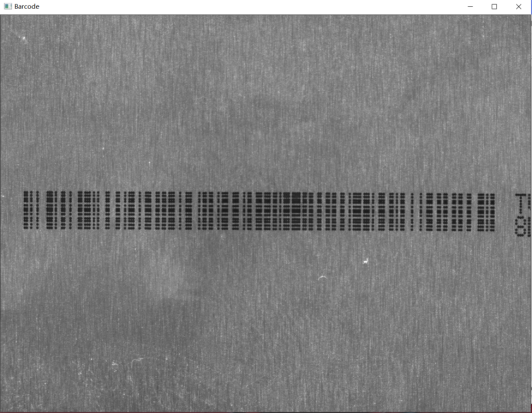
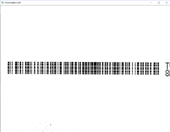
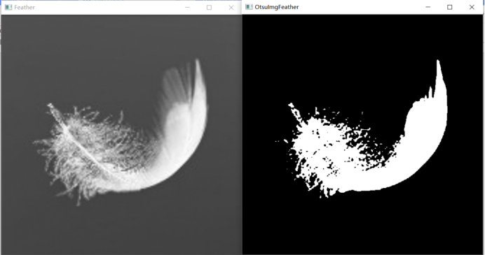
#阈值分割 通过设定不同的特征阈值，把图像像素点分为若干类
import cv2 as cv
#导入cv包

img1 = cv.imread("Feather.jpg", 0)
img2 = cv.imread("Barcode.jpg", 0)   #从E盘读取图片

th1, OtsuImgFeather = cv.threshold(img1, 0, 255, cv.THRESH_OTSU)
th2, OtsuImgBarcode = cv.threshold(img2, 0, 255, cv.THRESH_OTSU)  #遍历灰度0-255，选择一个灰度值
cv.imshow("Feather", img1)  #显示Feather图片
print(th1)  #输出0-255之间的树--阈值
cv.imshow("OtsuImgFeather", OtsuImgFeather)  #分割后的图片
cv.imshow("Barcode", img2)  #显示Barcode图片
print(th2)  #输出0-255之间的树--阈值
cv.imshow("OtsuImgBarcode", OtsuImgBarcode)  #分割后的图片
# 等待按键并销毁窗口
cv.waitKey()
cv.destroyAllWindows()

运行结果
138.0
85.0

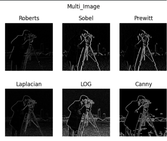
2、各类边缘检测算子

#2.各类边缘检测算子
import cv2
import numpy as np
import matplotlib.pyplot as plt
#导入要使用的各类包

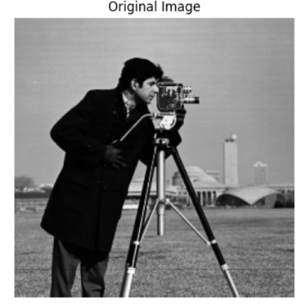
image = cv2.imread("Cameraman.tif")
image = cv2.cvtColor(image, cv2.COLOR_BGR2GRAY)  #读入图像并灰度化

# 自定义卷积核

# Roberts边缘算子--基于交叉差分的梯度算法
#利用局部差分算子寻找边缘的算子，采用对角线方向相邻两像素之差近似梯度幅值检测边缘
#Roberts算子的模板--水平方向
kernel_Roberts_x = np.array([
    [1, 0],
    [0, -1]
])
#Roberts算子的模板--竖直方向
kernel_Roberts_y = np.array([
    [0, -1],
    [1, 0]
])

# Sobel边缘算子--用于边缘检测的离散微分算子，结合了高斯平滑和微分求导
#根据图像边缘旁边明暗程度把该区域内超过某个数的特定点记为边缘
#Sobel算子的模板--水平方向
kernel_Sobel_x = np.array([
    [-1, 0, 1],
    [-2, 0, 2],
    [-1, 0, 1]])
#Sobel算子的模板--竖直方向
kernel_Sobel_y = np.array([
    [1, 2, 1],
    [0, 0, 0],
    [-1, -2, -1]])

# Prewitt边缘算子--图像边缘检测的微分算子
#利用特定区域内像素灰度值产生的差分视线边缘检测
#Prewitt算子的模板--竖直方向
kernel_Prewitt_x = np.array([
    [-1, 0, 1],
    [-1, 0, 1],
    [-1, 0, 1]])
#Prewitt算子的模板--水平方向
kernel_Prewitt_y = np.array([
    [1, 1, 1],
    [0, 0, 0],
    [-1, -1, -1]])

# 拉普拉斯卷积核
kernel_Laplacian_1 = np.array([
    [0, 1, 0],
    [1, -4, 1],
    [0, 1, 0]])
kernel_Laplacian_2 = np.array([
    [1, 1, 1],
    [1, -8, 1],
    [1, 1, 1]])
# 下面两个卷积核不具有旋转不变性
kernel_Laplacian_3 = np.array([
    [2, -1, 2],
    [-1, -4, -1],
    [2, 1, 2]])
kernel_Laplacian_4 = np.array([
    [-1, 2, -1],
    [2, -4, 2],
    [-1, 2, -1]])

# 5*5 LOG卷积模板
kernel_LoG = np.array([
    [0, 0, -1, 0, 0],
    [0, -1, -2, -1, 0],
    [-1, -2, 16, -2, -1],
    [0, -1, -2, -1, 0],
    [0, 0, -1, 0, 0]])


# Canny边缘检测 k为高斯核大小，t1,t2为阈值大小
def Canny(image, k, t1, t2):
    img = cv2.GaussianBlur(image, (k, k), 0)
    canny = cv2.Canny(img, t1, t2)
    return canny


# 卷积
output_1 = cv2.filter2D(image, -1, kernel_Roberts_x)
output_2 = cv2.filter2D(image, -1, kernel_Sobel_x)
output_3 = cv2.filter2D(image, -1, kernel_Prewitt_x)
output_4 = cv2.filter2D(image, -1, kernel_Laplacian_1)
output_5 = cv2.filter2D(image, -1, kernel_LoG)
output_6 = Canny(image, 3, 50, 150)

# 显示处理后的图像
plt.figure("Original Image")  # 图像窗口名称
plt.imshow(image, cmap='gray')  # 显示灰度图要加cmap
plt.axis('off')  # 关掉坐标轴为 off
plt.title('Original Image')  # 图像题目
plt.show()

plt.figure("Multi Image")  # 图像窗口名称
plt.suptitle('Multi_Image')  # 图片名称
plt.subplot(2, 3, 1), plt.title('Roberts')
plt.imshow(output_1, cmap='gray'), plt.axis('off')
plt.subplot(2, 3, 2), plt.title('Sobel')
plt.imshow(output_2, cmap='gray'), plt.axis('off')
plt.subplot(2, 3, 3), plt.title('Prewitt')
plt.imshow(output_3, cmap='gray'), plt.axis('off')
plt.subplot(2, 3, 4), plt.title('Laplacian')
plt.imshow(output_4, cmap='gray'), plt.axis('off')
plt.subplot(2, 3, 5), plt.title('LOG')
plt.imshow(output_5, cmap='gray'), plt.axis('off')
plt.subplot(2, 3, 6), plt.title('Canny')
plt.imshow(output_6, cmap='gray'), plt.axis('off')
plt.show()

# 等待按键并销毁窗口
cv2.waitKey()
cv2.destroyAllWindows()

运行结果

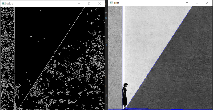
3、霍夫直线检测

#霍夫直线检测
#利用点与线的对偶性
import cv2
import numpy as np
#导入相关包
img = cv2.imread('BW_Art.jpg')

gray = cv2.cvtColor(img, cv2.COLOR_BGR2GRAY)  # 彩色图片灰度化
edges = cv2.Canny(gray, 100, 200)  # 执行边缘检测

cv2.imshow('edge', edges)  # 显示原始结果

# 执行Hough直线检测
#把在图像控件中的直线检测问题转换到参数空间中对点的检测问题，通过在参数空间里寻找峰值来完成直线检测任务
lines = cv2.HoughLines(edges, 1, np.pi / 180, 160)
lines1 = lines[:, 0, :]
for rho, theta in lines1:
    a = np.cos(theta)
    b = np.sin(theta)
    x0 = a * rho
    y0 = b * rho
    x1 = int(x0 + 1000 * (-b))
    y1 = int(y0 + 1000 * (a))
    x2 = int(x0 - 1000 * (-b))
    y2 = int(y0 - 1000 * (a))
    cv2.line(img, (x1, y1), (x2, y2), (255, 0, 0), 1)

cv2.imshow('line', img) #显示图片
#等待按键并销毁窗口
cv2.waitKey(0)
cv2.destroyAllWindows()

# 渐进概率式霍夫变换
img = cv2.imread('BW_Art.jpg')
gray = cv2.cvtColor(img, cv2.COLOR_BGR2GRAY)
edges = cv2.Canny(gray, 100, 200)

lines = cv2.HoughLinesP(edges, 1, np.pi/180, 30, minLineLength=200, maxLineGap=10)
lines = lines[:, 0, :]
for x1, y1, x2, y2 in lines:
    cv2.line(img, (x1, y1), (x2, y2), (255, 0, 0), 2)
cv2.imshow('img', img)
cv2.waitKey(0)
cv2.destroyAllWindows()

运行结果

实验小结

本次实验主要是这三个
1、阈值分割 通过设定不同的特征阈值，把图像像素点分为若干类
2、Roberts利用局部差分算子寻找边缘的算子，采用对角线方向相邻两像素之差近似梯度幅值检测边缘
3、Sobel边缘算子–用于边缘检测的离散微分算子，结合了高斯平滑和微分求导
根据图像边缘旁边明暗程度把该区域内超过某个数的特定点记为边缘
4、Prewitt边缘算子利用特定区域内像素灰度值产生的差分视线边缘检测
把在图像控件中的直线检测问题转换到参数空间中对点的检测问题，通过在参数空间里寻找峰值来完成直线检测任务
温馨提示
图片路径问题可自行更正