Machine Learning-Ex1（吴恩达课后习题） About Linear Regression

来源：吴恩达教授 教学视频课后题目

1. Simple MATLAB function

问题：输出一个5×5的单位矩阵

• MATLAB

warmUpExercise.m

function A = warmUpExercise()
A = eye(5);

lx.m

fprintf('Running warmUpExercise ... \n');
fprintf('5x5 Identity Matrix: \n');
warmUpExercise()

Running warmUpExercise ...

5x5 Identity Matrix:

ans =

1 0 0 0 0

0 1 0 0 0

0 0 1 0 0

0 0 0 1 0

0 0 0 0 1

---

• Python

inputIdentityMatrix.py

import numpy as np  # NumPy库支持大量的维度数组与矩阵运算

def inputIdentityMatrix():
    print(np.eye(5))

lx.py

from inputIdentityMatrix import *

inputIdentityMatrix()

[[1. 0. 0. 0. 0.]

[0. 1. 0. 0. 0.]

[0. 0. 1. 0. 0.]

[0. 0. 0. 1. 0.]

[0. 0. 0. 0. 1.]]

---

2. Linear regression with one variable

数据：

第一列：给出城市人口数量

第二列：该城市饭店的收益

2.1 Plotting the Data

• MATLAB

plotData.m

function plotData(x,y)
% r:red--x:用x作标记--MarkerSize:标记符的大小
plot(x,y,'rx', 'MarkerSize', 10); 
xlabel('Population of City in 10,000s');
ylabel('Profit in $10,000s');
title('Scatter plot of training data');
end

lx.m

fprintf('Plotting Data...\n')
data = load('ex1data1.txt');
X = data(:,1); % data第一列赋值给X向量
y = data(:,2); % data第二列赋值给y向量
m = length(X); % No. of training set

plotData(X,y);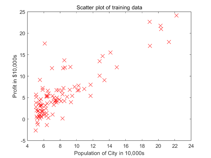

• Python

lx.py

import pandas as pd  # 一种用于数据分析的扩展程序库
import matplotlib.pyplot as plt  # matplotlib是一种数据可视化库

# header=None:无列标题行 names命名，data为DataFrame类型
# read_csv 以纯文本形式存储表格数据（数字和文本）
data = pd.read_csv('ex1data1.txt', header=None, names=['Population', 'Profit'])

# DataFrame类型与plot函数结合使用
data.plot(x='Population', y='Profit', kind='scatter', marker='x')
plt.show()  # 展示图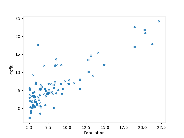

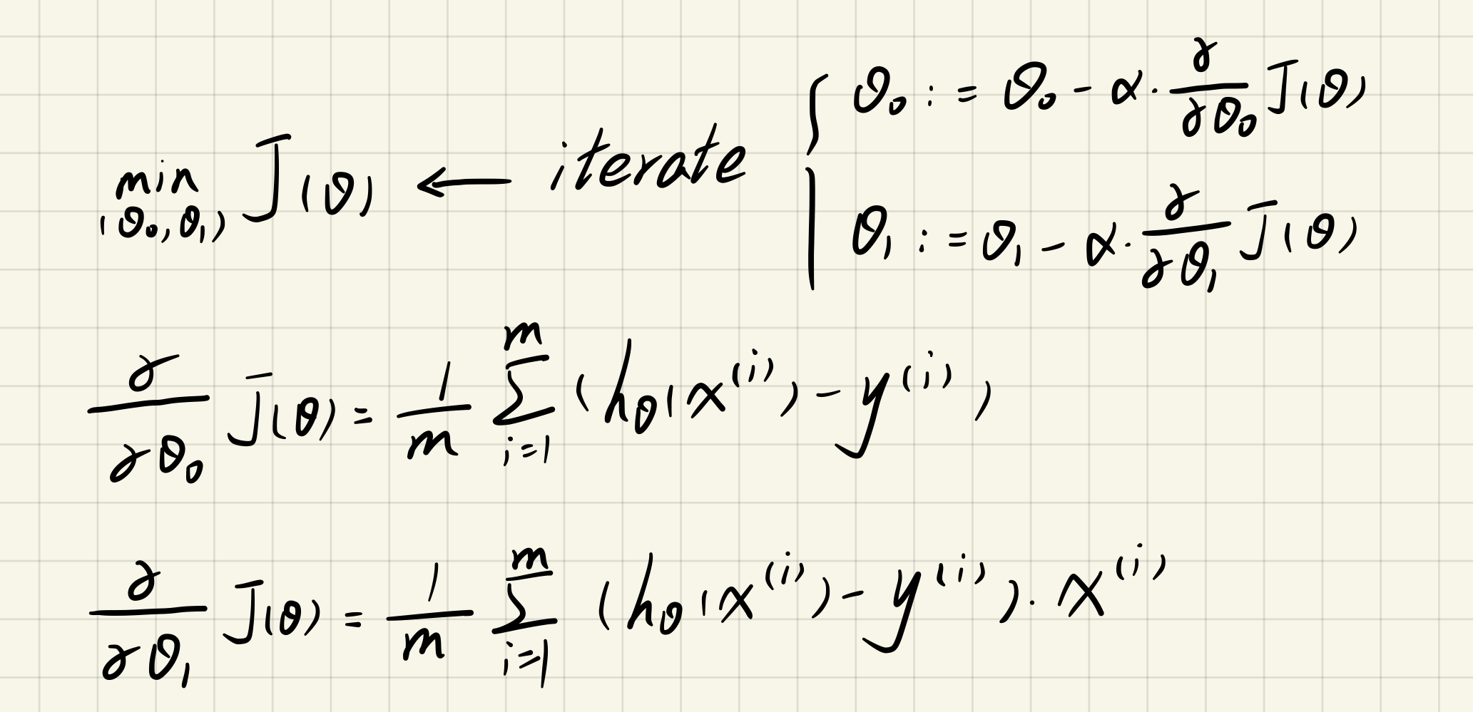
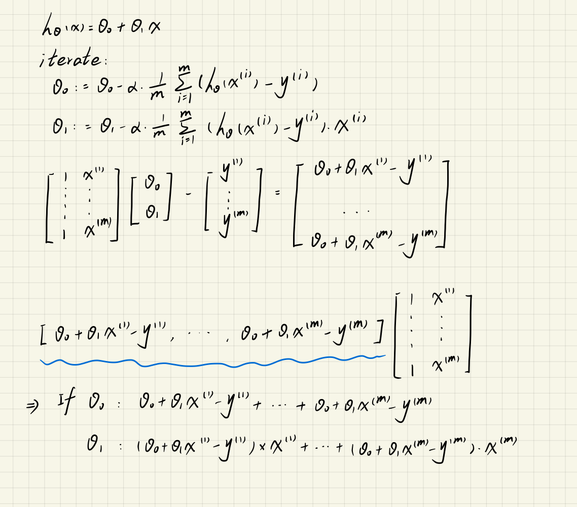
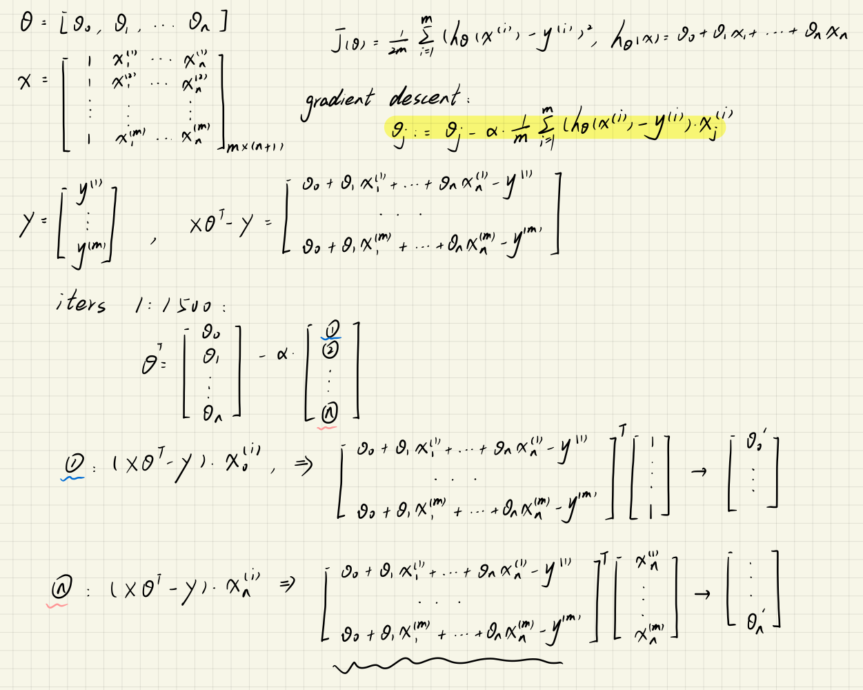
2.2 Gradient Descent

2.2.1 Update Equations

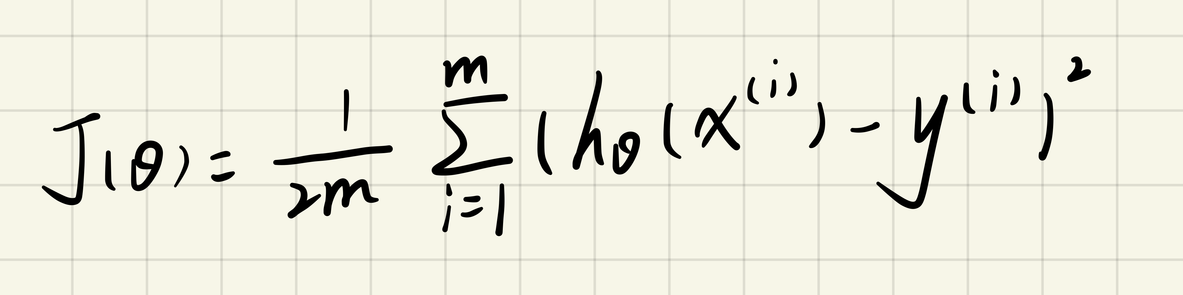
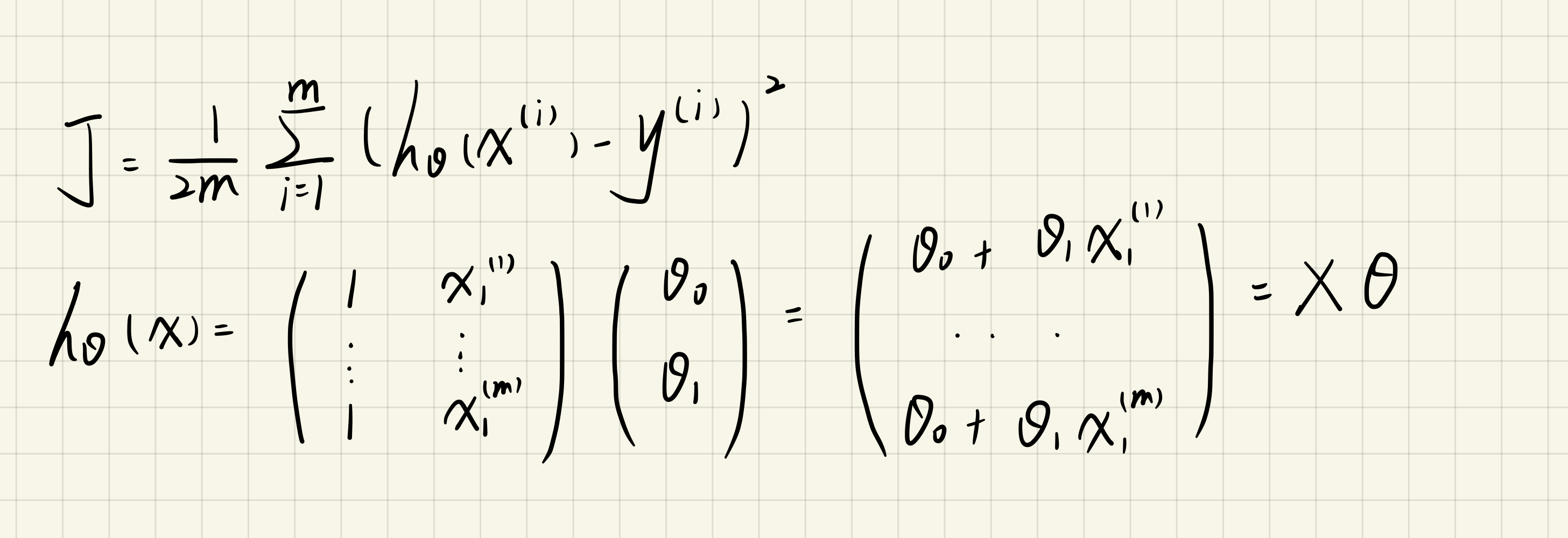
Cost Funtion：

Update Equations:

2.2.2 Computing the cost J(theta)

绘制J(theta)图像

• MATLAB

computeCost.m

function J = computeCost(X,y,theta)
predictions = X * theta; % 预测值
sqrErrors = (predictions - y).^2; % 误差的平方
J = 1 / (2 * length(X(:,1))) * sum(sqrErrors);
end

lx.m

data = load('ex1data1.txt');
m = length(data(:,1)); % No. of training set
X = [ones(m,1),data(:,1)]; % 设置X向量
y = data(:,2); % 设置y向量
theta = zeros(2,1); % theta设置为两行一列的0向量
alpha = 0.01; % learning rate 

fprintf('\nTesting the cost function ...\n');
J = computeCost(X,y,theta);
fprintf('With theta = [0 ; 0]\nCost computed = %f\n', J);

J = computeCost(X, y, [-1 ; 2]);
fprintf('\nWith theta = [-1 ; 2]\nCost computed = %f\n', J);

Testing the cost function ...

With theta = [0 ; 0]

Cost computed = 32.072734

With theta = [-1 ; 2]

Cost computed = 54.242455

---

• Python

lx.py

import pandas as pd  # 一种用于数据分析的扩展程序库
import numpy as np  # NumPy库支持大量的维度数组与矩阵运算
import matplotlib.pyplot as plt  # matplotlib是一种数据可视化库


def computeCost(theta, X, y):
    inner = np.power((X * theta.T - y), 2)
    # sum与np.sum的区别：sum不能处理二维及二维以上的数组
    return np.sum(inner) / (2 * len(X))


data = pd.read_csv('ex1data1.txt', header=None, names=['Population', 'Profit'])
data.insert(0, 'Ones', 1)  # 第0列插入名为Ones的值为1的一列
cols = data.shape[1]
X = data.iloc[:, :-1]  # iloc的用法[a:b,c:d]表示行从a到b-1，列从c到d-1
# data.shape[0]是行数
# data.shape[1]是列数
y = data.iloc[:, cols - 1:cols]

# 将X和y变成矩阵的形式
X = np.matrix(X)
y = np.matrix(y)
theta = np.matrix([0, 0])

# 观察维度
# print(X.shape, theta.shape, y.shape)  # (97, 2) (2, 1) (97, 1)

print(computeCost(theta, X, y))  # 32.072733877455676

2.2.3 Gradient descent

目的：通过改变theta的值，来最小化代价函数J(theta)。

• MATLAB

gradientDescent.m

function [theta,J_history] = gradientDescent(X,y,theta,alpha,num_iters)
m = length(y); % number of training examples
J_history = zeros(num_iters,1); % 设置代价函数J(theta)初始化为0

% 进入迭代
for iter = 1:num_iters
    theta_temp = theta; % 保证同时调整theta值
    for i = 1:length(theta) % 这里指theta0和theta1
        % 矩阵的转置可以用.'来表示，(:,i)即使用第i列
        theta_temp(i) = theta(i)-alpha/m*(X*theta-y).'*X(:,i);
    end
    theta = theta_temp;
    % 保存每一次迭代后代价函数的值
    J_history(iter) = computeCost(X,y,theta);
end
end

lx.m

data = load('ex1data1.txt');
m = length(data(:,1)); % No. of training set
X = [ones(m,1),data(:,1)]; % 设置X向量
y = data(:,2); % 设置y向量
theta = zeros(2,1); % theta设置为两行一列的0向量
alpha = 0.01; % learning rate 

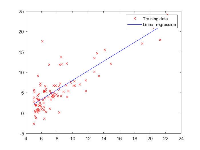
% 分布
plot(X(:,2),y,'rx');

num_iters = 1500;
theta = gradientDescent(X,y,theta,alpha,num_iters);
fprintf('Theta found by gradient descent:\n');
fprintf('%f\n',theta);

fprintf('Expected theta values (approx)\n');
fprintf(' -3.6303\n  1.1664\n\n');

hold on; % 后者可覆盖在前者图上
plot(X(:,2),X*theta,'b-');
legend('Training data', 'Linear regression')
hold off; % 关闭后，后者不可覆盖在前者图上

% Predict values for population sizes of 35,000 and 70,000
predict1 = [1,35000]*theta;
fprintf('For population = 35,000, we predict a profit of %f\n',predict1);
predict2 = [1,70000]*theta;
fprintf('For population = 70,000, we predict a profit of %f\n',predict2);

Theta found by gradient descent:

-3.630291

1.166362

Expected theta values (approx)

-3.6303

1.1664

For population = 35,000, we predict a profit of 40819.051970

For population = 70,000, we predict a profit of 81641.734232

• Python

Function.py

import numpy as np  # NumPy库支持大量的维度数组与矩阵运算


# 代价函数
def computeCost(theta, X, y):
    inner = np.power((X * theta.T - y), 2)
    # sum与np.sum的区别：sum不能处理二维及二维以上的数组
    return np.sum(inner) / (2 * len(X))


# 梯度下降
def gradientDescent(X, y, theta, iter_nums, alpha):
    X = np.matrix(X)
    y = np.matrix(y)
    # ravel用于将矩阵拉伸，shape[1]-返回列数
    temp_theta = np.matrix(np.zeros(theta.shape))  # temp_theta用于theta1和theta2同步进行更新
    para_nums = int(theta.ravel().shape[1])  # para_num为2，分别是theta0和theta1
    J_history = np.zeros(iter_nums)  # 用来记录每一次迭代后代价函数的值

    for i in range(iter_nums):
        inner = X * theta.T - y
        for j in range(para_nums):
            temp_theta[0, j] = theta[0, j] - (alpha / len(X)) * inner.T * X[:, j]
        theta = temp_theta
        J_history[i] = computeCost(theta, X, y)

    return theta, J_history

lx.py

import pandas as pd  # 一种用于数据分析的扩展程序库
import matplotlib.pyplot as plt  # matplotlib是一种数据可视化库
import numpy as np  # NumPy库支持大量的维度数组与矩阵运算
from Function import *

data = pd.read_csv('ex1data1.txt', header=None, names=['Population', 'Profit'])
data.insert(0, 'Ones', 1)  # 第0列插入名为Ones的值为1的一列
cols = data.shape[1]
X = data.iloc[:, :-1]  # iloc的用法[a:b,c:d]表示行从a到b-1，列从c到d-1
y = data.iloc[:, cols - 1:cols]
theta = np.matrix([0, 0])
alpha = 0.01
iter_nums = 1500

final_theta, Cost_J = gradientDescent(X, y, theta, iter_nums, alpha)

print('Theta found by gradient descent:')
print(final_theta)

# linspace(a,b,c)-将a-b区间分为c份
x = np.linspace(data.Population.min(), data.Population.max(), 100)
h_theta_ = final_theta[0, 0] + final_theta[0, 1] * x
# fig代表绘图窗口(Figure),ax代表此绘图窗口的坐标系(axis),subplots用于创建子图
fig, ax = plt.subplots()
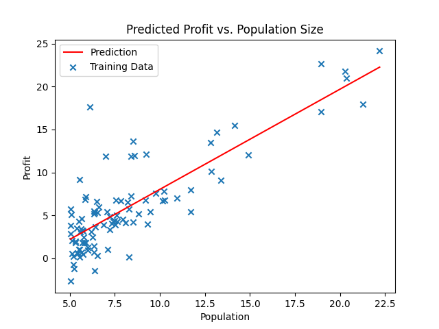
ax.plot(x, h_theta_, 'r', label='Prediction')

# Predict values for population sizes of 35,000 and 70,000
predict1 = [1, 35000] * final_theta.T
print('For population = 35,000, we predict a profit of %f' % predict1);
predict2 = [1, 70000] * final_theta.T
print('For population = 70,000, we predict a profit of %f' % predict2);

# 画出离散的点
ax.scatter(data.Population, data.Profit, marker='x', label='Training Data')
ax.legend(loc=2)  # loc位置，放在左上角
ax.set_xlabel('Population')
ax.set_ylabel('Profit')
ax.set_title('Predicted Profit vs. Population Size')
plt.show()

Theta found by gradient descent:

[[-3.63029144 1.16636235]]

For population = 35,000, we predict a profit of 40819.051970

For population = 70,000, we predict a profit of 81641.734232

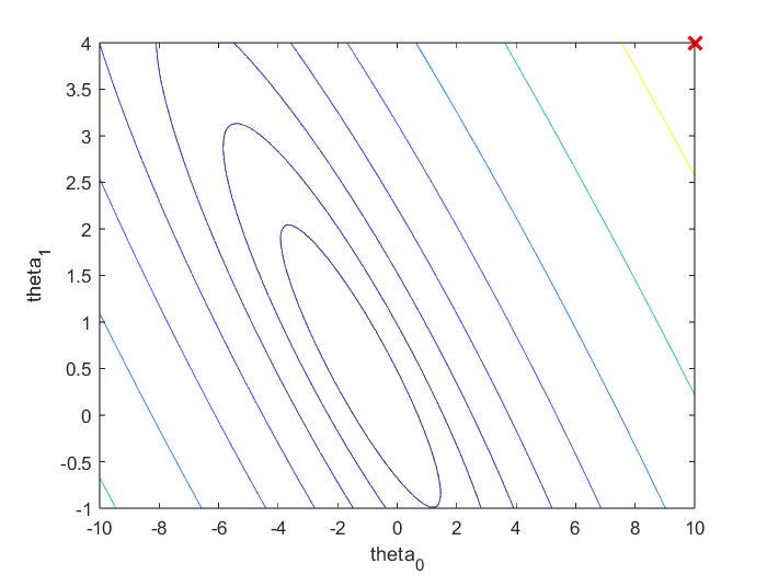
2.3 Visualizing J(theta)

关于：theta0、theta1不断变化时，J(theta)的变化

lx.m

data = load('ex1data1.txt');
m = length(data(:,1));
X = [ones(m,1),data(:,1)]; % 设置X向量
y = data(:,2); % 设置y向量

fprintf('Visualizing J(theta0, theta1) ...\n')

theta0_vals = linspace(-10,10,100);
theta1_vals = linspace(-1,4,100);
J_vals = zeros(length(theta0_vals),length(theta1_vals));

for i = 1:length(theta0_vals)
    for j = 1:length(theta1_vals)
        theta = [theta0_vals(i);theta1_vals(j)]; % 中间用分号表示列向量
        J_vals(i,j) = computeCost(X,y,theta);
    end
end

figure;
surf(theta0_vals,theta1_vals,J_vals);
xlabel('theta_0');
ylabel('theta_1');
figure;
contour(theta0_vals,theta1_vals,J_vals,logspace(-2, 3, 20));
xlabel('theta_0'); ylabel('theta_1');
hold on;
% theta此时为[10,4]
plot(theta(1), theta(2), 'rx', 'MarkerSize', 10, 'LineWidth', 2);
hold off;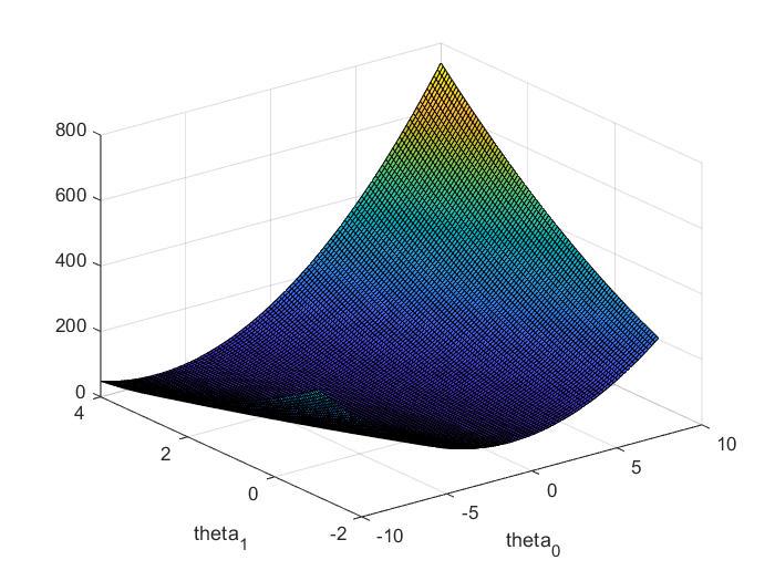

3. Linear regression with multiple variables（Python）

data：

column1	column2	column3
Size	Bedrooms	Price

3.1 Feature Normalization

目的：特征归一化，可以使梯度下降更快些收敛。

做法：(每类特征值-它的平均值)/标准差

featureScaling.py

def featureScaling(data):
    # mean()默认为mean(0)-列平均，mean(1)-行平均，std()-标准差
    return (data - data.mean()) / data.std()

main.py

import pandas as pd  # 一种用于数据分析的扩展程序库
from featureScaling import *  # 特征缩放

# 若数据中无列标题行，则需要执行header=None
data = pd.read_csv('ex1data2.txt', header=None, names=['Size', 'Bedrooms', 'Price'])
data = featureScaling(data)
print(data.head())

#        Size  Bedrooms     Price
# 0  0.130010 -0.223675  0.475747
# 1 -0.504190 -0.223675 -0.084074
# 2  0.502476 -0.223675  0.228626
# 3 -0.735723 -1.537767 -0.867025
# 4  1.257476  1.090417  1.595389

3.2 Gradient Descent

theta一定要同时迭代

computeCost.py

import numpy as np  # NumPy库支持大量的维度数组与矩阵运算

def computeCost(X, y, theta):
    return np.sum(np.power((X * theta.T - y), 2)) / (2 * len(X))

gradientDescent.py

import numpy as np  # NumPy库支持大量的维度数组与矩阵运算
from computeCost import *


def gradientDescent(X, y, theta, alpha, iters):
    cost = np.zeros(iters)
    theta_item = np.matrix(np.zeros(theta.shape))
    m = len(X)
    for i in range(iters):
        Errors = X * theta.T - y
        theta_item = theta - (alpha / len(X)) * Errors.T * X
        theta = theta_item
        cost[i] = computeCost(X, y, theta)
    return theta, cost

main.py

import pandas as pd  # 一种用于数据分析的扩展程序库
import numpy as np  # NumPy库支持大量的维度数组与矩阵运算
from featureScaling import *  # 特征缩放
from gradientDescent import *

# 若数据中无列标题行，则需要执行header=None
data = pd.read_csv('ex1data2.txt', header=None, names=['Size', 'Bedrooms', 'Price'])
data = featureScaling(data)
data.insert(0, 'Ones', 1)  # 在第0列添加名为Ones值为1的列向量

# 初始化X和y、theta
columns = data.shape[1]
X = data.iloc[:, 0:columns - 1]
y = data.iloc[:, columns - 1:columns]
X = np.matrix(X)
y = np.matrix(y)
theta = np.matrix(np.zeros(X.shape[1]))

alpha = 0.01  # learning rate
iters = 1500  # iterate

theta, cost = gradientDescent(X, y, theta, alpha, iters)
print("theta:")
print(theta)
print("cost:")
print(cost)

# theta:
# [[-1.11188321e-16  8.84042349e-01 -5.24551809e-02]]
# cost:
# [0.4805491  0.47198588 0.46366462 ... 0.13068671 0.13068671 0.13068671]

3.3 Normal Equation

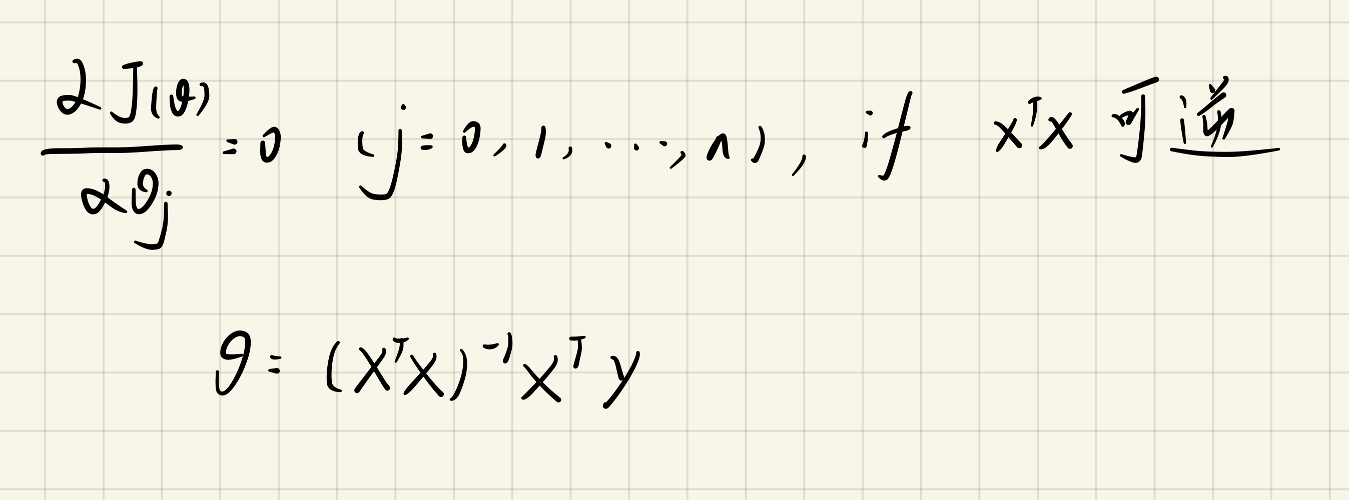
normalEquation.py

import numpy as np  # NumPy库支持大量的维度数组与矩阵运算

def normalEquation(X, y):
    # np.linalg.inv:求逆;np.linalg.pinv:求伪逆
    theta = np.linalg.inv(X.T * X) * X.T * y
    return theta

main.py

import pandas as pd  # 一种用于数据分析的扩展程序库
import numpy as np  # NumPy库支持大量的维度数组与矩阵运算
from featureScaling import *  # 特征缩放
from normalEquation import *  # 正规方程
from computeCost import *  # 代价函数

# 若数据中无列标题行，则需要执行header=None
data = pd.read_csv('ex1data2.txt', header=None, names=['Size', 'Bedrooms', 'Price'])
data = featureScaling(data)
data.insert(0, 'Ones', 1)  # 在第0列添加名为Ones值为1的列向量

# 初始化X和y、theta
columns = data.shape[1]
X = data.iloc[:, 0:columns - 1]
y = data.iloc[:, columns - 1:columns]
X = np.matrix(X)
y = np.matrix(y)
theta = normalEquation(X, y)
print("theta:")
print(theta)
cost = computeCost(X, y, theta.T)
print("Cost:")
print(cost)
# theta:
# [[-1.11022302e-16]
#  [ 8.84765988e-01]
#  [-5.31788197e-02]]
# Cost:
# 0.13068648053904192