吴恩达机器学习配套第一次编程练习（代码+学习记录）（Octave/Matlab）

吴恩达机器学习配套编程练习第一周（Octave/Matlab）

本文仅供个人学习记录，尽量写的详细，可供参考

（注：吴恩达课程的练习只需要再他所给的一个个函数文件中增添代码，最后运行‘主函数（ex.m）’文件即可

%% Machine Learning Online Class - Exercise 1: Linear Regression

%  Instructions
%  ------------
% 
%  This file contains code that helps you get started on the
%  linear exercise. You will need to complete the following functions 
%  in this exericse:
%
%     warmUpExercise.m
%     plotData.m
%     gradientDescent.m
%     computeCost.m
%     gradientDescentMulti.m
%     computeCostMulti.m
%     featureNormalize.m
%     normalEqn.m
%
%  For this exercise, you will not need to change any code in this file,
%  or any other files other than those mentioned above.
%
% x refers to the population size in 10,000s
% y refers to the profit in $10,000s
%

注释介绍如图，大概就包括了上面几个Octave函数文件，本次分为两个任务，第一个是单变量的线性线性回归和多变量线性回归，其主文件对应作业包中的ex1.m和ex1_multi.m

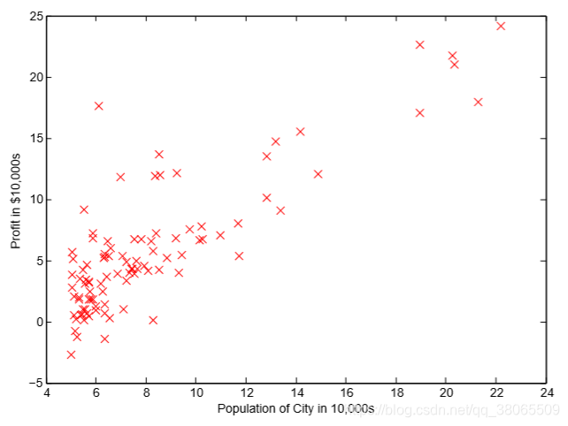
首先第一步利用他所提供的数据文件，进行图片绘制

%% ======================= Part 2: Plotting =======================
fprintf('Plotting Data ...\n')
data = load('ex1data1.txt');
X = data(:, 1); y = data(:, 2);
m = length(y); % number of training examples

% Plot Data
% Note: You have to complete the code in plotData.m
plotData(X, y);

读取文件用X存第一列数据，y存第二列，m为训练集的个数，最后调用plotData函数，如图

function plotData(x, y)

    figure; % open a new figure window
    plot(x, y, 'rx', 'MarkerSize', 10); % Plot the data
    ylabel('Profit in $10,000s'); % Set the y   axis label
    xlabel('Population of City in 10,000s'); % Set the x   axis label

end

其中可能不明白意思我解释一下plot中 ‘rx’表示用红色的叉叉来描点，然后markersize标记大小为10

画出来大概这样

接着我们要运行梯度下降算法来找出一条直线拟合这些数据，来看主函数体中的第二步要求我们做什么

%% =================== Part 3: Gradient descent ===================
fprintf('Running Gradient Descent ...\n')

X = [ones(m, 1), data(:,1)]; % Add a column of ones to x
theta = zeros(2, 1); % initialize fitting parameters

% Some gradient descent settings
iterations = 1500;
alpha = 0.01;

% compute and display initial cost
computeCost(X, y, theta)

% run gradient descent
theta = gradientDescent(X, y, theta, alpha, iterations);

% print theta to screen
fprintf('Theta found by gradient descent: ');
fprintf('%f %f \n', theta(1), theta(2));

其中我们只需要修改computeCost和gradientDescent函数即可

function J = computeCost(X, y, theta)

    J = 0;

    J = sum((X * theta - y).^2) / (2*m);     % X(79,2)  theta(2,1)

end

对应公式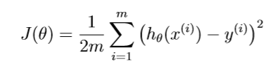应该不难写出

再看gradientDescent函数

function [theta, J_history] = gradientDescent(X, y, theta, alpha, num_iters)

% Initialize some useful values
m = length(y); % number of training examples
J_history = zeros(num_iters, 1);


for iter = 1:num_iters
    theta(1) = theta(1) - alpha / m * sum(X * theta_s - y);       
    theta(2) = theta(2) - alpha / m * sum((X * theta_s - y) .* X(:,2));	

 
    J_history(iter) = computeCost(X, y, theta);

end
J_history %打印显示

end

同样根据课上所讲的梯度下降公式，对应公式直接写出来，进行num_iters次的迭代不断更新theta并且再J_history中记录下每次迭代的Cost。接着我们开始绘图

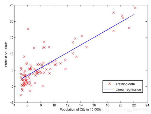
% Plot the linear fit
hold on; % keep previous plot visible
plot(X(:,2), X*theta, 'g-')
legend('Training data', 'Linear regression')
hold off % don't overlay any more plots on this figure

成功拟合训练集数据的直线大概长这样

接着我们就需要用两个新数据来预测下

% Predict values for population sizes of 35,000 and 70,000
predict1 = [1, 3.5] *theta;
fprintf('For population = 35,000, we predict a profit of %f\n',
    predict1*10000);
predict2 = [1, 7] * theta;
fprintf('For population = 70,000, we predict a profit of %f\n',
    predict2*10000);

fprintf('Program paused. Press enter to continue.\n');
pause;

运行之后得到结果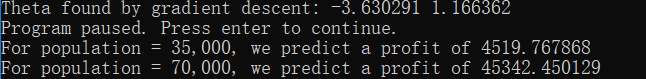

预测数据成功

最后我们用三维图像和等高线来可视化J函数（数学意义上的函数）看看，注意函数的参数应该是theta0和theta1

%% ============= Part 4: Visualizing J(theta_0, theta_1) =============
fprintf('Visualizing J(theta_0, theta_1) ...\n')

% Grid over which we will calculate J
theta0_vals = linspace(-10, 10, 100);%linespace讲-10到10分成100等分，也就是一个1X100的行向量
theta1_vals = linspace(-1, 4, 100);%类似

% initialize J_vals to a matrix of 0's
J_vals = zeros(length(theta0_vals), length(theta1_vals));%初始化一个空的J_vals矩阵

% Fill out J_vals
for i = 1:length(theta0_vals)
    for j = 1:length(theta1_vals)
	  t = [theta0_vals(i); theta1_vals(j)];    
	  J_vals(i,j) = computeCost(X, y, t);%对每一个theta0 theta1进行代价计算并记录
    end
end


% Because of the way meshgrids work in the surf command, we need to 
% transpose J_vals before calling surf, or else the axes will be flipped
J_vals = J_vals';%转置，surf函数的要求。
% Surface plot
figure;
surf(theta0_vals, theta1_vals, J_vals)
xlabel('\theta_0'); ylabel('\theta_1');

% Contour plot 等高线绘制，看看就行了，吴恩达的作业要求也只是要我们看懂就行，如果函数不懂的可以用help XXX来查阅
figure;
% Plot J_vals as 15 contours spaced logarithmically between 0.01 and 100
contour(theta0_vals, theta1_vals, J_vals, logspace(-2, 3, 20))
xlabel('\theta_0'); ylabel('\theta_1');
hold on;
plot(theta(1), theta(2), 'rx', 'MarkerSize', 10, 'LineWidth', 20);

我把解释写在了代码中，最后绘图结果：

单变量的线性回归就这样了，其实多变量的线性回归很类似