


引言(水字数。。。)
在当今生物信息学领域,随着高通量测序技术的飞速发展,我们能够获得大量的基因组数据。这些数据为研究病原微生物的毒力因子提供了宝贵的资源。然而,如何从海量的基因序列中准确预测出毒力因子,仍然是一个巨大的挑战。本文将介绍一种基于pipeline的基因类型预测方法,旨在提高毒力因子预测的准确性和效率。
怎么构建一个ML|DL的pipeline实现序列预测呢,首先要明确步骤,数据准备》特征提取》模型搭建》模型验证优化等
一、数据来源和预处理
数据来源和预处理,决定了你训练模型的下限,在当下AI这么火的情况下,模型优化仅仅是锦上添花。
数据来源
我的数据来自deepvf论文公开的数据集,分为阳性和阴性,数据量:阳性:3000 阴性:4334
example:
>0|0|tr|A0A0E8T5Q1|A0A0E8T5Q1_STREE
MNNGYSPTSSNQQNVSVEHDIIMRGRRIIDITGVKQVESFDSEEFLLETVMGFLTIRGQNLQMKNLDVEKGIVSIKGKVNEMLYIDENQGEKTKGFFSKLFK
解释一下这段数据:(这里不需要知道太多,做模型仅仅需要知道你的每条数据和对应的标签是什么,后续构建相关关系让模型学就行)
标题行:每条序列的开头包含一行标题,包含一些标识信息,例如:序号或类别信息:0|1,可能用于标记不同的分组或类别。数据库标识符: gi|218561911|ref|YP_002343690.1|,这是基因信息数据库(如NCBI GenBank)中的ID,gi指“Gene Info Identifier”,ref表明该序列为参考序列,后面的YP_002343690.1是具体的参考ID。
序列部分:标题行之后是实际的氨基酸序列,以单字母代码(如M, I, G, D等)表示每个氨基酸残基。该序列描述了毒力因子的蛋白质序列,用于了解其在生物体中如何起作用。例如:MIGDMNELLLKSVEV... 和 MFGNSYGGYLANLCA... 是不同蛋白质的氨基酸序列。每个氨基酸在蛋白质中的特定位置影响其结构和功能,序列的完整性可以帮助预测其可能的生物活性。
数据预处理
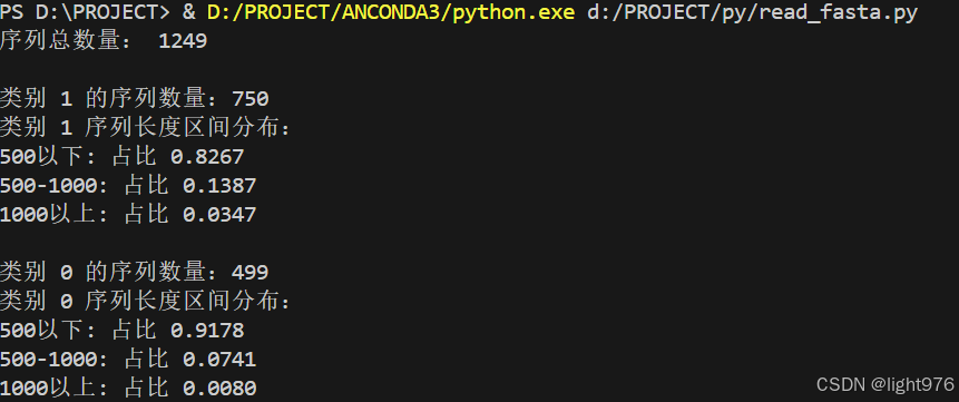
查看数据分布
OK了解完数据之后,我们需要进行一系列预处理,首先我们要知道数据分布大概是什么,通过这个代码,统计文件中各个阴性阳性样本数量,再根据序列长度来看看数据分布是什么样的,个人觉得不同序列长度数据的域差距不小。
import os
import re
import sys
from collections import Counter
import matplotlib.pyplot as plt

def readFasta(file):
    if os.path.exists(file) == False:
        print('Error: "' + file + '" does not exist.')
        sys.exit(1)

    with open(file) as f:
        records = f.read()

    if re.search('>', records) == None:
        print('The input file seems not in fasta format.')
        sys.exit(1)

    records = records.split('>')[1:]
    myFasta = []
    for fasta in records:
        array = fasta.split('\n')
        name, sequence = array[0].split()[0], re.sub('[^ARNDCQEGHILKMFPSTWYV-]', '-', ''.join(array[1:]).upper())
        myFasta.append([name, sequence])
    return myFasta

def classify_by_label(fastas):
    classified_fasta = {}
    for fasta in fastas:
        label = fasta[0].split("|")[1]  # 假设 label 在描述行的特定位置
        if label not in classified_fasta:
            classified_fasta[label] = []
        classified_fasta[label].append(fasta)
    return classified_fasta

def calculate_length_distribution(fastas):
    lengths = [len(fasta[1]) for fasta in fastas]
    length_counter = Counter(lengths)
    total_sequences = len(fastas)
    distribution = {length: count / total_sequences for length, count in length_counter.items()}
    return distribution

def categorize_lengths(distribution):
    categories = {
        '500以下': 0,
        '500-1000': 0,
        '1000以上': 0
    }
    for length, ratio in distribution.items():
        if length < 500:
            categories['500以下'] += ratio
        elif 500 <= length < 1000:
            categories['500-1000'] += ratio
        else:
            categories['1000以上'] += ratio
    return categories

def plot_stacked_bar_chart(classified_categories):
    labels = list(classified_categories.keys())
    categories = ['500以下', '500-1000', '1000以上']

    # 初始化数据
    data = {category: [] for category in categories}
    for label, categories_dict in classified_categories.items():
        for category in categories:
            data[category].append(categories_dict.get(category, 0))

    # 创建堆积柱状图
    fig, ax = plt.subplots(figsize=(10, 6))
    bottom = [0] * len(labels)
    colors = ['blue', 'green', 'red']

    for idx, category in enumerate(categories):
        ax.bar(labels, data[category], bottom=bottom, label=category, color=colors[idx])
        bottom = [b + d for b, d in zip(bottom, data[category])]

    # 添加数据标签
    for label_idx, label in enumerate(labels):
        for category_idx, category in enumerate(categories):
            value = data[category][label_idx]
            if value > 0:
                ax.text(label_idx, sum(data[cat][label_idx] for cat in categories[:category_idx+1]) - value / 2,
                        f'{value:.2%}', ha='center', va='center', color='white')

    # 设置标题和标签
    ax.set_xlabel('类别')
    ax.set_ylabel('占比')
    ax.set_title('各类别序列长度分布')
    ax.legend(title='长度区间')

    # 显示图表
    plt.show()

if __name__ == '__main__':
    fastas = readFasta(r'D:\PROJECT\py\PreVFs-RG-main\data\val.fasta')
    print("序列总数量:", len(fastas))

    # 根据类别分类
    classified_fasta = classify_by_label(fastas)

    # 统计每个类别的序列长度分布
    classified_categories = {}
    for label, fastas in classified_fasta.items():
        print(f"\n类别 {label} 的序列数量:{len(fastas)}")
        length_distribution = calculate_length_distribution(fastas)
        length_categories = categorize_lengths(length_distribution)
        classified_categories[label] = length_categories

        # 打印分类结果
        print(f"类别 {label} 序列长度区间分布:")
        for category, ratio in length_categories.items():
            print(f"{category}: 占比 {ratio:.4f}")

    # 绘制堆积柱状图
    plot_stacked_bar_chart(classified_categories)
数据集划分
然后要划分训练集和验证集,为什么我这里要提前划分好,而不直接用函数来随机划分。因为随机划分特征随机,训练出来的模型泛化性很差。这里附上划分代码
import os
import re
import sys
from collections import defaultdict
import random

def readFasta(file):
    if not os.path.exists(file):
        print(f'Error: "{file}" does not exist.')
        sys.exit(1)

    with open(file) as f:
        records = f.read()

    if re.search('>', records) is None:
        print('The input file seems not in fasta format.')
        sys.exit(1)

    records = records.split('>')[1:]
    myFasta = []
    for fasta in records:
        array = fasta.split('\n')
        name, sequence = array[0].split()[0], re.sub('[^ARNDCQEGHILKMFPSTWYV-]', '-', ''.join(array[1:]).upper())
        myFasta.append([name, sequence])
    return myFasta

def categorize_by_length(fastas):
    categories = defaultdict(list)
    for fasta in fastas:
        length = len(fasta[1])
        if length < 500:
            categories['500以下'].append(fasta)
        elif 500 <= length < 1000:
            categories['500-1000'].append(fasta)
        else:
            categories['1000以上'].append(fasta)
    return categories

def split_train_test(categories, test_ratio=0.2):
    train_set = []
    test_set = []
    for category, fastas in categories.items():
        random.shuffle(fastas)
        split_index = int(len(fastas) * (1 - test_ratio))
        train_set.extend(fastas[:split_index])
        test_set.extend(fastas[split_index:])
    return train_set, test_set

def save_fasta(fastas, file_path):
    with open(file_path, 'w') as f:
        for name, sequence in fastas:
            f.write(f'>{name}\n{sequence}\n')

if __name__ == '__main__':
    # 指定多个 FASTA 文件路径
    fasta_files = [
        r'D:\PROJECT\py\PreVFs-RG-main\data\train-balance.fasta'
    ]

    # 读取所有 FASTA 文件
    all_fastas = []
    for file in fasta_files:
        all_fastas.extend(readFasta(file))

    print("总序列数量:", len(all_fastas))

    # 按序列长度分类
    categorized_fastas = categorize_by_length(all_fastas)

    # 等比划分训练集和测试集
    train_set, test_set = split_train_test(categorized_fastas)

    print("训练集序列数量:", len(train_set))
    print("测试集序列数量:", len(test_set))

    # 保存为 FASTA 文件
    save_fasta(train_set, r'D:\PROJECT\py\PreVFs-RG-main\data\train.fasta')
    save_fasta(test_set, r'D:\PROJECT\py\PreVFs-RG-main\data\test.fasta')

    print("训练集和测试集已保存为 FASTA 文件。")
二、选择特征提取方法
划分完成之后,需要考虑特征提取方法。
这里我用的是AAC,在序列预测非常常用的一种方法
AAC 方法是一种计算序列中每种氨基酸出现频率的特征提取方法,主要描述氨基酸的整体组成。
原理:统计每种氨基酸在整个序列中出现的比例,即:
特征向量:特征向量的维度为 20,因为氨基酸有 20 种标准类型,AAC 向量直接反映序列中每种氨基酸的相对丰度。
优点:AAC 提取方法简单且计算效率高,提供了序列的整体氨基酸组成信息。某些毒力因子可能有特定的氨基酸偏好,这种方法可以帮助识别这些偏好。
应用:AAC 特征在毒力因子、抗性基因、功能蛋白等预测任务中是一个基础的特征,尤其适用于对序列的初步筛选分析。
| 0 | # | A | C | D | E | F | G | H |
| 1 | 0|1|gi|115534244|ref|YP_783826.1| | 0.044944 | 0 | 0.039326 | 0.044944 | 0.117978 | 0.067416 | 0.02809 |
| 2 | 0|1|gi|16802734|ref|NP_464219.1| | 0.074434 | 0.004854 | 0.058252 | 0.110032 | 0.035599 | 0.053398 | 0.022654 |
| 3 | 0|1|gi|16802625|ref|NP_464110.1| | 0.126556 | 0.002075 | 0.029046 | 0.043568 | 0.014523 | 0.074689 | 0.010373 |
| 4 | 0|1|gi|16803640|ref|NP_465125.1| | 0.085873 | 0.00831 | 0.052632 | 0.091413 | 0.033241 | 0.072022 | 0.01385 |
这是我提取出来的案例,不用想太多这个问题,理解成每个字母的概率分布就行。
三、模型构建
选择好提取特征方法后,我们来构建一个pipeline基于随机森林实现毒力因子预测。
from Bio import SeqIO
from sklearn.model_selection import StratifiedKFold
from sklearn.preprocessing import LabelEncoder
from sklearn.ensemble import RandomForestClassifier
from sklearn.metrics import classification_report, accuracy_score
from sklearn.pipeline import Pipeline
from sklearn.feature_selection import SelectKBest, f_classif
import numpy as np
# 1. 读取fasta文件
def read_fasta(file_paths):
sequences = []
labels = []
for file_path in file_paths:
for record in SeqIO.parse(file_path, "fasta"):
seq = str(record.seq)
label = record.description.split("|")[1] # 假设label在标题的特定位置
sequences.append(seq)
labels.append(label)
return sequences, labels
# 2. 特征提取方法(AAC)
def aac_feature_extraction(sequences):
aac_features = []
for seq in sequences:
aac = [seq.count(aa) / len(seq) for aa in "ACDEFGHIKLMNPQRSTVWY"]
aac_features.append(aac)
return np.array(aac_features)
# 3. 标签编码与处理
def preprocess_labels(labels):
label_encoder = LabelEncoder()
labels = label_encoder.fit_transform(labels)
return labels
# 4. 构建机器学习Pipeline
def build_pipeline():
pipeline = Pipeline([
('select_k_best', SelectKBest(f_classif, k=100)), # 特征选择
('classifier', RandomForestClassifier(random_state=42)) # 分类器
])
return pipeline
# 5. 训练和评估Pipeline
def train_and_evaluate_pipeline(train_fasta_file, test_fasta_file, feature_method, num_classes, cv=10):
# 读取训练数据
train_sequences, train_labels = read_fasta([train_fasta_file])
X_train = aac_feature_extraction(train_sequences)
y_train = preprocess_labels(train_labels)
# 读取测试数据
test_sequences, test_labels = read_fasta([test_fasta_file])
X_test = aac_feature_extraction(test_sequences)
y_test = preprocess_labels(test_labels)
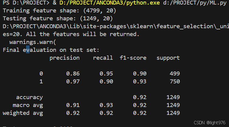
print("Training feature shape:", X_train.shape)
print("Testing feature shape:", X_test.shape)
pipeline = build_pipeline()
skf = StratifiedKFold(n_splits=cv, shuffle=True, random_state=42)
scores = []
pipeline.fit(X_train, y_train)
y_pred = pipeline.predict(X_test)
print("Final evaluation on test set:")
print(classification_report(y_test, y_pred))
print(f"Test accuracy: {accuracy_score(y_test, y_pred):.4f}")
# 运行 Pipeline
train_fasta_file = r"D:\PROJECT\py\PreVFs-RG-main\data\train.fasta"
test_fasta_file = r"D:\PROJECT\py\PreVFs-RG-main\data\val.fasta"
feature_method = "aac"
num_classes = 2 # 类别数量
train_and_evaluate_pipeline(train_fasta_file, test_fasta_file, feature_method, num_classes)最后结果达到的精度如下,感觉数据划分对这个结果影响非常大,第一我选的随机划分时结果在0.68左右,后期自己根据序列长度和阴性阳性按比例划分后,精度为0.92。所以说数据处理这部分决定了结果的下限。
最后附上数据链接:DeepVF | Download Page (monash.edu)


 被折叠的 条评论
为什么被折叠?
被折叠的 条评论
为什么被折叠?
 到【灌水乐园】发言


