多模态学习路线（2）——DL基础系列

目录

前言

一、归一化

1. Layer Normalization (LN)

2. Batch Normalization (BN) 

3. Instance Normalization (IN) 

4. Group Normalization (GN)

5. Root Mean Square Normalization（RMSNorm）

二、激活函数

1. Sigmoid激活函数（二分类）

2. Tanh激活函数

3. ReLU

4. Leaky Relu / PeLU (α不可学习 / 可学习)

5. Softmax激活函数（多分类）

三、优化器

1. SGD

2. BGD

3. MBGD-Mini-batch GD

4. Momentum

5. Adam

6. AdamW（Adam + Weight Decay)​​​

四、损失函数

1. ​​L1 Loss（MAE）

2. L2 Loss（MSE）

3. ​​BCE Loss（二元交叉熵，Binary Cross-Entropy）

4. CE Loss（多元交叉熵 / 交叉熵，Cross-Entropy）

5. KL散度（Kullback-Leibler Divergence）

6. ​​Focal Loss（二分类，类别不平衡）

7. InfoNCE Loss

五、注意力机制

1. Self Attention 与 Cross Attention

2. 双向Attention 与 Casual Attention

3. Sclaed Dot-Product Attention 与 Multi-Head Attention（MHA）

4. 分组查询注意力（Grouped-Query Attention, GQA）​​

5. 多层注意力（Multi-Level Attention, MLA）​

6. 多查询注意力（Multi-Query Attention, MQA）​

六、位置编码(正余弦PE，ROPE，RPE，ROPE+ 2D RPE)

1. 绝对位置编码(正余弦位置编码)

2. 旋转位置编码（ROPE）

七、Decoder解码

1. Greedy Search

2. Beam Search

3. Temperature Sampling

4. Top-k Sampling（手撕）

5. Top-p Sampling（手撕）

八、NLP、CV、AIGC、MLLMs经典算法

1. NLP

2. CV

3. AIGC

4. MLLMs

---

前言

一、归一化：Layer Normalization (LN)、Batch Normalization (BN)、Instance Normalization (IN)、Group Normalization (GN)、Root Mean Square Normalization（RMSNorm）；

二、激活函数：sigmoid，Tanh，ReLU，Leaky ReLU，Softmax；

三、优化器：SGD，BGD，MBGD-Mini-batch GD，Momentum，Adam，AdamW；

四、损失函数：​​L1 Loss（MAE），​​L2 Loss（MSE），BCE Loss（二元交叉熵，Binary Cross-Entropy），​​交叉熵（多元交叉熵，Cross-Entropy），KL散度（Kullback-Leibler Divergence），Focal Loss（二分类，类别不平衡），InfoNCE Loss​​；

五、注意力机制：Self Attention 与 Cross Attention，双向Attention 与 Casual Attention，Scaled Dot-Product Attention 与 Multi-Head Attention（MHA），分组查询注意力（GQA），多层注意力（MLA），多查询注意力（MQA）；

六、位置编码：绝对位置编码（正余弦位置编码），旋转位置编码（ROPE），相对位置编码（PRE），RoPE（文本）+ 2D RPE（视觉）；

七、Decoder解码：Greedy Search，Beam-Search，Temperature Sampling，Top-k Sampling，Top-p Sampling；

八、NLP、CV、AIGC、MLLMs经典算法

---

一、归一化

1. Layer Normalization (LN)

输入：(N, L, D);

计算：N不变，对每个样本上的(L, D)求总体均值和方差；

### 输入：(batch_size, seq_len, feature_dim)（常见于序列模型Transformer/RNN）
def layernorm(x, gamma, beta, eps=1e-5):
    # x shape: (N, L, D)
    N = x.shape[0]
    mean = np.mean(x, axis=(1, 2)).reshape(N, 1, 1)  # (N, 1, 1)
    var = np.var(x, axis=(1, 2)).reshape(N, 1, 1)    # (N, 1, 1)
    x_normalized = (x - mean) / np.sqrt(var + eps)   # 归一化
    return gamma * x_normalized + beta 

### e.g. x形状为 (2, 3, 4)（batch_size=2, seq_len=3, feature_dim=4）
x = [
    [ # 样本 1
        [1, 2, 3, 4],  # seq_len1
        [5, 6, 7, 8],  # seq_len2
        [9, 10, 11, 12] # seq_len3
    ],
    [ # 样本 2
        [-1, -2, -3, -4],  # seq_len1
        [-5, -6, -7, -8],  # seq_len2
        [-9, -10, -11, -12] # seq_len3
    ]
]
x = np.array(x)
gamma, beta = 0.1, 0.1
x_ln = layernorm(x, gamma, beta, eps=1e-5)
print(x_ln.shape)
"""
LN 计算：对样本1归一化：计算所有时间步和特征的均值
mean = (1+2+...+12) / 12 = 6.5
var = (1²+2²+...+12²)/12 - mean² = 11.9167
样本2同理（每个样本独立计算）。
"""

• Adaptive LayerNorm：对传统 LayerNorm 的增强，通过引入可学习的缩放（γ）和偏移（β）参数，使得归一化过程能够根据输入数据的不同进行调整，从而提高了模型的灵活性和表现。这种方法尤其适用于多任务学习和多模态学习等复杂任务，可以更好地适应不同的数据分布，提高训练的稳定性和效率。

class AdaptiveLayerNorm(nn.Module):
    def __init__(self, input_dim):
        super(AdaptiveLayerNorm, self).__init__()
        # 可学习的缩放和偏移参数
        self.gamma = nn.Parameter(torch.ones(input_dim))
        self.beta = nn.Parameter(torch.zeros(input_dim))
    def forward(self, x):
        # 计算均值和方差
        mean = x.mean(dim=-1, keepdim=True)
        var = x.var(dim=-1, keepdim=True, unbiased=False)
        # 归一化
        x_norm = (x - mean) / torch.sqrt(var + 1e-5)
        # 自适应缩放和偏移
        return self.gamma * x_norm + self.beta

2. Batch Normalization (BN) 

输入：(N, C, H, W)；

计算：C不变，对每个C上的(N, H, W)求总体均值和方差；

# 输入x：(batch_size, channels, height, width)（常见于CNN）
def batchnorm(x, gamma, beta, eps=1e-5):
    # x shape: (N, C, H, W)
    c = x.shape[1]
    mean = np.mean(x, axis=(0, 2, 3)).reshape(1,c,1,1)  # 计算每个通道的均值，维度 (1,C,1,1)
    var = np.var(x, axis=(0, 2, 3)).reshape(1,c,1,1)   # 计算每个通道的方差，维度 (1,C,1,1)
    x_normalized = (x - mean) / np.sqrt(var + eps)  # 归一化
    return gamma * x_normalized + beta  # 缩放和偏移

# e.g. x形状为 (2, 3, 2, 2)（batch_size=2, channels=3, height=2, width=2）
x = [
    [  # 样本 1
        [[1, 2], [3, 4]],  # 通道 1
        [[5, 6], [7, 8]],  # 通道 2
        [[9, 10], [11, 12]] # 通道 3
    ],
    [  # 样本 2
        [[-1, -2], [-3, -4]],  # 通道 1
        [[-5, -6], [-7, -8]],  # 通道 2
        [[-9, -10], [-11, -12]] # 通道 3
    ]
]
x = np.array(x)
gamma, beta = 0.1, 0.1
x_bn = batchnorm(x, gamma, beta, eps=1e-5)
print(x_bn.shape)
"""
对通道1归一化：计算所有样本和空间位置的均值. 
mean = (1+2+3+4 + (-1-2-3-4)) / 8 = 0
var = (1²+2²+...+(-4)²)/8 - mean² = 7.5
其他通道类似（每个通道独立计算）。
"""

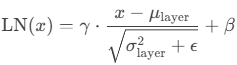
3. Instance Normalization (IN) 

输入：(N, C, H, W)；

计算：(N, C)不变，对每个(N, C)上的(H, W)求总体均值和方差；

def instance_norm(x, gamma, beta, eps=1e-5):
    # x shape: (N, C, H, W)
    N, C = x.shape[0], x.shape[1] 
    mean = np.mean(x, axis=(2, 3)).reshape(N, C, 1, 1)  # 计算每个样本每个通道的均值，维度 (N, C)
    var = np.var(x, axis=(2, 3)).reshape(N, C, 1, 1)   # 计算方差，维度 (N, C)
    x_normalized = (x - mean) / np.sqrt(var + eps)  # 归一化
    return gamma * x_normalized + beta  # 缩放和偏移

# 形状为 (2, 3, 2, 2)（batch=2, channels=3, height=2, width=2）：
x = [
    [ # 样本 1
        [[1, 2], [3, 4]],  # 通道 1
        [[5, 6], [7, 8]],  # 通道 2
        [[9, 10], [11, 12]] # 通道 3
    ],
    [ # 样本 2
        [[-1, -2], [-3, -4]],  # 通道 1
        [[-5, -6], [-7, -8]],  # 通道 2
        [[-9, -10], [-11, -12]] # 通道 3
    ]
]
x = np.array(x)
gamma, beta = 0.1, 0.1
x_in = instance_norm(x, gamma, beta, eps=1e-5)
print(x_in.shape)
"""
对样本1的通道1归一化：
mean = (1+2+3+4)/4 = 2.5
var = [(1-2.5)² + (2-2.5)² + (3-2.5)² + (4-2.5)²]/4 = 1.25
其他通道和样本同理（每个样本的每个通道独立计算）。
"""

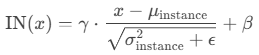
4. Group Normalization (GN)

输入：(N, C, H, W), group nums=G；

输出：(N, C, H, W) --> (N, G, C//G, H, W) --> (N, C, H, W)

计算：(N, G)不变，对每个(N, G)上的(C//G, H, W)求总体均值和方差；

# 核心思想：将通道分组，对每个样本的每组通道归一化，解决小 batch 下 BN 不稳定的问题，适用于检测、分割等任务。
def group_norm(x, gamma, beta, G, eps=1e-5):
    # x shape: (N, C, H, W) 或 (N, C, L)
    # G: 分组数（如 C=32, G=8 → 每组 4 个通道）
    N, C, H, W = x.shape[0], x.shape[1], x.shape[2], x.shape[3]
    x = np.reshape(x, (N, G, C//G, H, W))  # 分组后形状 (N, G, C/G, H, W)
    mean = np.mean(x, axis=(2, 3, 4)).reshape(N, G)  # 计算每组均值，维度 (N, G)
    var = np.var(x, axis=(2, 3, 4)).reshape(N, G)   # 计算每组方差，维度 (N, G)
    x_normalized = (x - mean) / np.sqrt(var + eps)  # 归一化
    x_normalized = np.reshape(x_normalized, (N, C, H, W))  # 恢复原始形状
    return gamma * x_normalized + beta  # 缩放和偏移

# x形状为 (2, 4, 2, 2)（batch=2, channels=4, height=2, width=2），分组数 G=2
x = [
    [ # 样本 1
        [[1, 2], [3, 4]],  # 通道 1 (组 1)
        [[5, 6], [7, 8]],  # 通道 2 (组 1)
        [[9, 10], [11, 12]], # 通道 3 (组 2)
        [[13, 14], [15, 16]] # 通道 4 (组 2)
    ],
    [ # 样本 2
        [[-1, -2], [-3, -4]],  # 通道 1 (组 1)
        [[-5, -6], [-7, -8]],  # 通道 2 (组 1)
        [[-9, -10], [-11, -12]], # 通道 3 (组 2)
        [[-13, -14], [-15, -16]] # 通道 4 (组 2)
    ]
]
x = np.array(x)
gamma, beta = 0.1, 0.1
x_gn = group_norm(x, gamma, beta, G=2, eps=1e-5)
print(x_gn.shape)
"""
GN 计算（G=2，每组 2 个通道）：
对样本 1 的组 1（通道 1+2）归一化：
mean = (1+2+3+4 + 5+6+7+8)/8 = 4.5
var = [(1-4.5)² + ... + (8-4.5)²]/8 = 5.25
组 2（通道 3+4）和其他样本同理。
"""

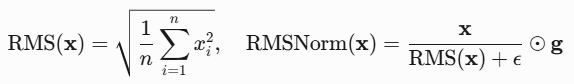
5. Root Mean Square Normalization（RMSNorm）

传统LN计算均值和方差；RMSNorm去除均值中心化，仅使用均方根RMS进行缩放。避免减法，提高数值稳定性，简化计算；仅使用均方根RMS归一化，计算量更小。只对特征维度(feature_dim)计算。

# (batch_size, seq_len, feature_dim)
def rms_norm(x, gamma, eps=1e-5):
    rms = np.sqrt(np.mean(x**2, axis=-1, keepdims=True))  # 只在特征维度（D）计算
    return gamma * x / (rms + eps)

# x形状为 (2, 3, 4)
x = [
    [[1, 2, 3, 4], [5, 6, 7, 8], [9, 10, 11, 12]],  # 样本1
    [[-1, -2, -3, -4], [-5, -6, -7, -8], [-9, -10, -11, -12]]  # 样本2
]
x = np.array(x)
gamma = 1.0
x_rms = rms_norm(x, gamma, eps=1e-5)
print(x_rms.shape)

"""
对样本1的第一个时间步 [1, 2, 3, 4] 计算：
RMS = sqrt(1**2 + 2**2 + 3**2 + 4**2)/4 = sqrt(7.5) ≈ 2.7386
归一化后：
[1,2,3,4]/2.7386 ≈ [0.3651,0.7303,1.0954,1.4606]
最终输出（γ=1）：与归一化值相同。
"""

方法	归一化维度	依赖 Batch	适用场景	python实现
Layer Norm (LN)	(C, H, W) 或 (L, D)	否	Transformer/RNN	torch.nn.LayerNorm()
Batch Norm (BN)	(N, H, W)	是	CNN（大 batch）	torch.nn.BatchNorm2d()
Instance Norm (IN)	(H, W)（单样本单通道）	否	风格迁移、图像生成	torch.nn.InstanceNorm2d()
Group Norm (GN)	(G, C//G, H, W)	否	小 batch 检测/分割（如 Mask R-CNN）	torch.nn.GroupNorm()

归一化	公式	计算量	适用场景
LN	(x−μ)/σ * γ	较高（需均值）	RNN/Transformer序列模型
BN	(x−μ)/σ * γ	高（依赖batch，需维护running mean/var）	CNN、CV任务
RMSNorm	x/RMS * γ	较低	大模型（如LLaMA）

二、激活函数

        激活函数实际是神经网络中的一种非线性变换，使神经网络能够捕捉到非线性关系，从而更好地逼近复杂的函数或映射。

        大模型常用的激活函数包括ReLU、Leaky ReLU、ELU、Swish和GELU。ReLU计算简单且有效避免梯度消失问题，加快训练速度，但可能导致神经元死亡；Leaky ReLU通过引入小斜率缓解ReLU的缺点；GeLU一种改进的ReLU函数，可以提供更好的性能和泛化能力；Swish一种自门控激活函数，可以提供非线性变换，并具有平滑和非单调的特性，在平滑性和性能上表现优异，但计算开销较大。

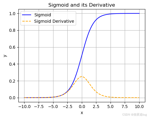
1. Sigmoid激活函数（二分类）

• 特点：输出范围(0,1)，适合二分类输出层，但易导致梯度消失。

import numpy as np
import matplotlib.pyplot as plt

def sigmoid(x):
    return 1 / (1 + np.exp(-x))

x = np.linspace(-5, 5, 100)
y = sigmoid(x)
plt.plot(x, y)
plt.title("Sigmoid")
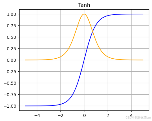
plt.show()

2. Tanh激活函数

• 输出范围(-1,1)，梯度比Sigmoid更强，但仍存在梯度消失。

import numpy as np
import matplotlib.pyplot as plt

def relu(x):
    return np.maximum(0, x)
x = np.linspace(-5, 5, 100)
y = relu(x)
plt.plot(x, y)
plt.title("ReLU")
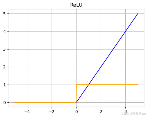
plt.show()

3. ReLU

•  输出范围([0, +♾️)，计算高效，缓解梯度消失，但可能导致“神经元死亡”（负输入梯度为0）。

import numpy as np
import matplotlib.pyplot as plt

def relu(x):
    return np.maximum(0, x)
x = np.linspace(-5, 5, 100)
y = relu(x)
plt.plot(x, y)
plt.title("ReLU")
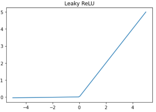
plt.show()

4. Leaky Relu / PeLU (α不可学习 / 可学习)

• 输出范围(-♾️, +♾️)，引入小的负斜率（α），缓解“神经元死亡”问题。

import numpy as np
import matplotlib.pyplot as plt

def leaky_relu(x, alpha=0.01):
    return np.where(x >= 0, x, alpha * x)

x = np.linspace(-5, 5, 100)
y = leaky_relu(x)
plt.plot(x, y)
plt.title("Leaky ReLU")
plt.show()

5. Softmax激活函数（多分类）

• 将输出转化为概率分布，适用于多分类输出层。

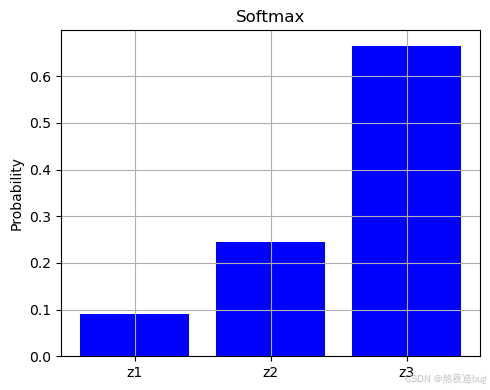
import numpy as np
import matplotlib.pyplot as plt

def softmax(x):
    exp_x = np.exp(x - np.max(x))  # 防溢出
    return exp_x / np.sum(exp_x, axis=0)

x = np.array([1.0, 2.0, 3.0])
print(softmax(x))  # 输出: [0.09003057 0.24472847 0.66524096]
"""
np.exp(x - np.max(x))通过减去输入向量x的最大值（x - np.max(x)），
可以保证：所有指数部分的输入(xi−max(x))≤0​​，因此exi−max(x)的范围是(0,1]，
避免exi的爆炸性增长，同时不改变softmax的输出结果。
（数学上等价：分子分母同时除以np.exp(max(x))，和原来等价）。
"""

三、优化器

优化器分类	优化器	核心思想	优点	缺点
基础梯度下降类	BGD	全批量梯度更新	稳定收敛	计算成本高
	SGD	单样本随机更新	计算快	噪声大
	MBGD	小批量梯度更新	平衡速度与稳定性	需调批量大小
动量类	Momentum	历史梯度加权平均	加速收敛，减少震荡	需调动量系数
自适应学习率类	Adam	自适应动量 + 学习率	适合大多数场景	内存占用高
	AdamW	Adam + 权重衰减	更稳定的权重衰减	超参更多

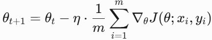
1. SGD

目标​​：每次迭代​​随机选择一个样本​​计算梯度，更新参数。​​更新公式​​如下，其中 (xi​,yi​) 是随机选择的样本。

​​特点​：计算快，但噪声大，收敛不稳定。

2. BGD

目标​​：在每次迭代中使用​​全部训练样本​​计算损失函数的梯度，更新参数。更新公式如下，其中，η是学习率，∇θ​J(θ)是损失函数J对参数θ的梯度（所有样本的平均梯度）。

特点：全局最优解，但计算成本高，不适合大规模数据。

3. MBGD-Mini-batch GD

目标​​：每次迭代使用​​一个小批量（Mini-batch）​​样本计算梯度。​​更新公式如下，其中，m是批量大小。

​​特点​​：平衡了BGD的稳定性和SGD的速度。

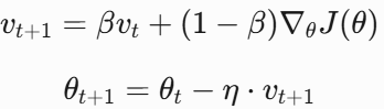
4. Momentum

​​目标​​：引入动量项（指数加权平均梯度）加速收敛，减少震荡。更新公式如下，其中，β是动量系数（通常0.9）。

​​推导​​：动量本质是对历史梯度的加权平均，帮助参数在梯度方向一致时加速，不一致时减速。

5. Adam

目标​​：结合动量（一阶矩）和自适应学习率（二阶矩）。

特点：收敛快。主流选择，适用于大多数任务。

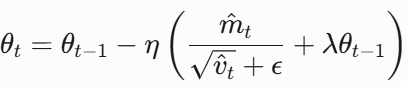
6. AdamW（Adam + Weight Decay)​​​

​​改进点​​：将权重衰减（L2正则化）从梯度更新中解耦，直接加到参数上。更新公式如下，其中，λ是权重衰减系数。

特点：Adam的权重衰减会因自适应学习率被缩放，AdamW则直接应用衰减，更稳定。

四、损失函数

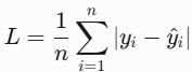
1. ​​L1 Loss（MAE）

• 原理：预测值与真实值的绝对误差，对异常值不敏感（鲁棒性强）；
• 公式

import numpy as np

def l1_loss(y_true, y_pred):
    return np.mean(np.abs(y_true - y_pred))

y_true, y_pred = 1.0, 0.9
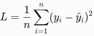
print(round(l1_loss(y_true, y_pred), 4))

2. L2 Loss（MSE）

• 原理​​：计算预测值与真实值的平方误差，对异常值敏感（放大误差）;
• 公式

import numpy as np

def l2_loss(y_true, y_pred):
    return np.mean((y_true - y_pred) ** 2)

y_true, y_pred = 1.0, 0.9
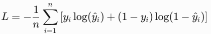
print('l2 loss(mse): ', round(l2_loss(y_true, y_pred), 4))

3. ​​BCE Loss（二元交叉熵，Binary Cross-Entropy）

• ​​原理​​：二分类任务的交叉熵，输出通过Sigmoid压缩到[0,1]概率；
• 公式

# BCE Loss二元交叉熵（二分类）
def binary_cross_entropy(y_true, y_pred, epsilon=1e-7):
    """
    y_true : 真实标签0或1
    y_pred : 预测概率，经过Sigmoid）后的概率分布
    epsilon : 极小值，防止log(0)数值错误
    """
    y_pred = np.clip(y_pred, epsilon, 1 - epsilon)
    return -np.mean(y_true * np.log(y_pred) + (1 - y_true) * np.log(1 - y_pred))
y_true = np.array([1, 1, 0])   # 真实值/label: 1, 1, 0
y_pred = np.array([0.9, 0.8, 0.6])   # 预测的概率分布: 0.9(1), 0.8(1), 0.6(1)，最后一个预测错误
print("bce Loss:", round(binary_cross_entropy(y_true, y_pred), 4))
"""
np.clip(y_pred, epsilon, 1 - epsilon)   
(1) ​​防止数值不稳定，通过clip将y_pred限制在[eps, 1-eps]内；
(2)​​避免梯度消失或爆炸。
"""

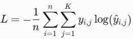
4. CE Loss（多元交叉熵 / 交叉熵，Cross-Entropy）

• 原理​​：衡量预测概率分布与真实分布的差异，用于多分类任务，输出通过Softmax压缩到概率分布。
• ​​公式​​（多分类）

# CE Loss多元交叉熵/交叉熵（多分类）
def cross_entropy(y_true, y_pred, eps=1e-15):
    """
    y_true : 真实标签0或1
    y_pred : 预测概率，经过Sigmoid）后的概率分布
    epsilon : 极小值，防止log(0)数值错误
    """
    y_pred = np.clip(y_pred, eps, 1 - eps)
    return -np.mean(np.sum(y_true * np.log(y_pred), axis=1))
y_true = np.array([
    [1, 0, 0],  # Class 0
    [0, 1, 0],  # Class 1
    [0, 0, 1],  # Class 2
    [0, 1, 0]   # Class 1
])
# 预测的概率分布，输出经过softmax转为概率分布
y_pred = np.array([
    [0.7, 0.2, 0.1],  # class 0
    [0.1, 0.6, 0.3],  # class 1
    [0.2, 0.3, 0.5],  # class 2
    [0.4, 0.5, 0.1]   # class 1
])
print('cross_entropy交叉熵: ', round(cross_entropy(y_true, y_pred), 4))
"""
np.clip(y_pred, eps, 1 - eps) 
(1)​​防止数值不稳定，通过clip将y_pred限制在[eps, 1-eps]内；
(2)​​避免梯度消失或爆炸​。
"""

5. KL散度（Kullback-Leibler Divergence）

• 原理​​：衡量两个概率分布 P 和 Q 之间的差异，非对称且非负；
• 公式

  

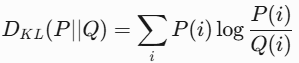
import numpy as np

def kl_divergence(p, q):
    p = np.clip(p, 1e-10, 1)   #  # 避免log(0)的情况；保证数值稳定；防止梯度消失和梯度爆炸
    q = np.clip(q, 1e-10, 1)
    return np.sum(p * np.log(p / q))

# 示例
p = np.array([0.1, 0.4, 0.5])
q = np.array([0.3, 0.3, 0.4])
print("KL Divergence: ", round(kl_divergence(p, q), 4))

6. ​​Focal Loss（二分类，类别不平衡）

• 原理​​：解决不平衡的二类别问题，输出通过Sigmoid压缩到[0,1]概率。通过权重α和聚焦参数γ，减少易分类样本的损失贡献，解决类别不平衡问题。
• ​​公式​​（二分类）

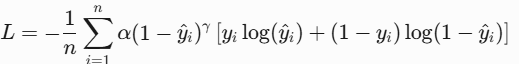
import numpy as np

def focal_loss(y_true, y_pred, alpha=0.25, gamma=2.0):
    y_pred = np.clip(y_pred, 1e-8, 1 - 1e-8)
    loss = -alpha * (1 - y_pred) ** gamma * (y_true * np.log(y_pred) + (1 - y_true) * np.log(1 - y_pred))
    return np.mean(loss)

y_true = np.array([1, 0, 1, 0, 1])  # 真实二类别标签
y_pred = np.array([0.9, 0.1, 0.8, 0.2, 0.7])  # 预测概率分布0.9(1), 0.1(0), 0.8(1), 0.2(0), 0.7(1)

loss = focal_loss(y_true, y_pred)
print(f"Focal Loss: ", round(loss, 4))

7. InfoNCE Loss

• 原理​​：对比学习中的损失函数，最大化正样本对的相似度，最小化负样本对的相似度；
• ​​公式​​：其中τ是温度系数。

import torch
import torch.nn as nn
import torch.nn.functional as F
import numpy as np
np.random.seed(42)
torch.manual_seed(42)


# PyTorch 实现
def infonce_loss_torch(query, positive_key, negative_keys, temperature=1.0):
    """
    Args:
        query: (batch_size, embedding_size)
        positive_key: (batch_size, embedding_size)
        negative_keys:(num_negative, embedding_size)
    """
    positive_logits = torch.sum(query * positive_key, dim=1, keepdim=True) # (batch_size, 1)
    negative_logits = torch.matmul(query, negative_keys.t())  # (batch_size, num_negative)
    logits = torch.cat([positive_logits, negative_logits], dim=1)  # (batch_size, 1 + num_negative)
    
    # Compute cross-entropy loss (positive sample is at index 0)
    labels = torch.zeros(query.size(0), dtype=torch.long, device=query.device)
    loss = F.cross_entropy(logits / temperature , labels)
    return loss

# Numpy 实现
def infonce_loss_numpy(query, positive_key, negative_keys, temperature=1.0):
    """
    Args:
        query: (batch_size, embedding_size)
        positive_key: (batch_size, embedding_size)
        negative_keys:(num_negative, embedding_size)
    """
    positive_logits = np.sum(query * positive_key, axis=1, keepdims=True) / temperature  # (batch_size, 1)
    negative_logits = np.dot(query, negative_keys.T) / temperature  # (batch_size, num_negative)
    logits = np.concatenate([positive_logits, negative_logits], axis=1)  # (batch_size, 1 + num_negative)
    
    labels = np.zeros(query.shape[0], dtype=np.int64)  # positive sample is at index 0
    exp_logits = np.exp(logits - np.max(logits, axis=1, keepdims=True))  # numerical stability
    softmax_probs = exp_logits / np.sum(exp_logits, axis=1, keepdims=True)
    loss = -np.mean(np.log(softmax_probs[:, 0] + 1e-8))  # avoid log(0)
    return loss


# 定义参数，生成随机数据
batch_size, num_negative, embedding_size = 32, 36, 512
query = np.random.randn(batch_size, embedding_size)
positive_key = np.random.randn(batch_size, embedding_size)
negative_keys = np.random.randn(num_negative, embedding_size)
# 归一化
query = query / np.linalg.norm(query, axis=1, keepdims=True)
positive_key = positive_key / np.linalg.norm(positive_key, axis=1, keepdims=True)
negative_keys = negative_keys / np.linalg.norm(negative_keys, axis=1, keepdims=True)
query_torch = torch.from_numpy(query)
positive_key_torch = torch.from_numpy(positive_key)
negative_keys_torch = torch.from_numpy(negative_keys)

loss_torch = infonce_loss_torch(query_torch, positive_key_torch, negative_keys_torch)
print(f"InfoNCE loss（PyTorch）: {loss_torch.item():.4f}")
loss_numpy = infonce_loss_numpy(query, positive_key, negative_keys)
print(f"InfoNCE loss（Numpy）: {loss_numpy: 4f}")

五、注意力机制

​​类型​​	​​Q/K/V来源​​	是否共享参数	典型应用​​
Self Attention（手撕）	同序列	否	BERT文本编码
Cross Attention	Q来自A序列，K/V来自B	否	机器翻译、多模态
双向Attention	全面捕捉上下文信息	是	需要全局理解的场景（BERT）
Causal Attention	同序列+三角掩码	否	GPT文本生成
MHA（手撕）	同序列，多组独立	否	通用Transformer
GQA	Q分组，组内共享K/V	部分共享	Llama 2等大模型
MQA	多Q，共享K/V	是（K/V共享）	轻量级模型推理
MLA	捕获不同粒度的特征	是	长文档处理、层次化结构建模（如Hierarchical Transformer）

1. Self Attention 与 Cross Attention

• Self Attention
  • ​​原理​​：计算序列中每个位置与其他位置的关联权重，生成上下文感知的表示。公式如，其中 Q,K,V 来自同一输入序列。
  • 特点​​：捕捉序列内部依赖关系，无方向性限制。
  • 应用​​：Transformer的核心组件，适用于文本/图像等序列数据（如BERT、ViT）。

• Cross Attention​
  • ​​原理​​：一个序列的Q与另一序列的K,V交互，例如解码器关注编码器输出。
  • ​​特点​​：建立跨序列关系（如源语言到目标语言）。
  • ​​应用​​：机器翻译（Seq2Seq）、多模态融合（文本-图像对齐）。

2. 双向Attention 与 Casual Attention

• 双向Attention
  • ​​原理​​：自注意力的特例，允许每个位置同时关注前后文（无方向限制）。
  • ​​特点​​：全面捕捉上下文信息。
  • ​​应用​​：需要全局理解的场景（如BERT的预训练）。
• Casual Attention
  • 原理​​：通过掩码限制当前位置仅关注之前的位置（未来信息不可见）。
  • ​​特点​​：保证自回归生成的时序性。
  • ​​应用​​：文本生成（如GPT）、自回归模型。

3. Sclaed Dot-Product Attention 与 Multi-Head Attention（MHA）

• Sclaed Dot-Product Attention（常考手撕）

import torch
import torch.nn as nn
import torch.nn.functional as F
import math
import numpy as np
np.random.seed(42)
torch.manual_seed(42)

class DotProductAttention(nn.Module):
    def __init__(self, d_model):
        super().__init__()
        self.scale = math.sqrt(d_model)

    def forward(self, q, k, v, mask=None):
        scores = torch.matmul(q, k.transpose(-2, -1)) / self.scale
        if mask is not None:
            scores = scores.masked_fill(mask == 0, -1e9)
        weights = F.softmax(scores, dim=-1)
        output = torch.matmul(weights, v)
        return output, weights


batch_size, seq_len, d_model = 4, 12, 512
attn = DotProductAttention(d_model)
q = torch.randn(batch_size, seq_len, d_model)
k = v = torch.randn(batch_size, seq_len, d_model)  # 简单起见，k和v相同
output, weights = attn(q, k, v)
print(f"输入: q{k.shape}, k{k.shape}, v{v.shape}")
print(f"输出: {output.shape}, 权重形状: {weights.shape}")
print("第一个样本的注意力权重:\n", weights[0].detach().numpy().round(3))

• Multi-Head Attention（MHA）
  • ​​原理​​：将 Q,K,V 投影到多个子空间，并行计算多个自注意力头，拼接后融合如下，每个头关注不同方面的特征。
  • ​​特点​​：增强模型捕捉多样化模式的能力。
  • ​​应用​​：几乎所有Transformer变体（如GPT、BERT）。

    

• MHA手撕代码（常考手撕）

import torch
import torch.nn as nn
import torch.nn.functional as F

class MultiHeadAttention(nn.Module):
    def __init__(self, dim, n_head, dropout=0.1):
        super(MultiHeadAttention, self).__init__()
        self.dim = dim
        self.head_dim = dim // n_head
        self.n_head = n_head
        assert self.dim == self.head_dim * n_head
        self.linear_q = nn.Linear(dim, dim)
        self.linear_k = nn.Linear(dim, dim)
        self.linear_v = nn.Linear(dim, dim)
        self.dropout = nn.Dropout(dropout)
        self.fc_out = nn.Linear(dim, dim)

    def forward(self, x, mask=None):
        b, t, d = x.size()
        Q = self.linear_q(x)
        K = self.linear_k(x)
        V = self.linear_v(x)
        
        # Reshape and transpose for multi-head attention
        Q = Q.view(b, t, self.n_head, self.head_dim).transpose(1, 2)
        K = K.view(b, t, self.n_head, self.head_dim).transpose(1, 2)
        V = V.view(b, t, self.n_head, self.head_dim).transpose(1, 2)
        
        # Scaled dot-product attention
        score = torch.matmul(Q, K.transpose(2, 3)) / torch.sqrt(torch.tensor(self.head_dim, dtype=torch.float32))
        
        # Apply mask (for decoder)
        if mask is not None:
            mask = mask.unsqueeze(1)  # Add head dimension
            score = score.masked_fill(mask == 0, -1e9)
        
        # Softmax and dropout
        score = F.softmax(score, dim=-1)
        if self.dropout is not None:
            score = self.dropout(score)
        
        # Combine heads and project back to original dimension
        output = torch.matmul(score, V).transpose(1, 2).contiguous().view(b, t, d)
        output = self.fc_out(output)
        return output

def generate_mask(len_seq):
    """生成下三角掩码矩阵（用于Decoder的自回归掩码）"""
    return torch.tril(torch.ones(len_seq, len_seq)).bool()

# 示例用法
embed_dim = 512
num_heads = 8
model = MultiHeadAttention(embed_dim, num_heads)
x = torch.randn(16, 10, 512)  # 输入形状: [batch_size, seq_len, dim]
mask = generate_mask(10).unsqueeze(0).expand(16, 10, 10)  # 扩展掩码到batch维度
output = model(x, mask)
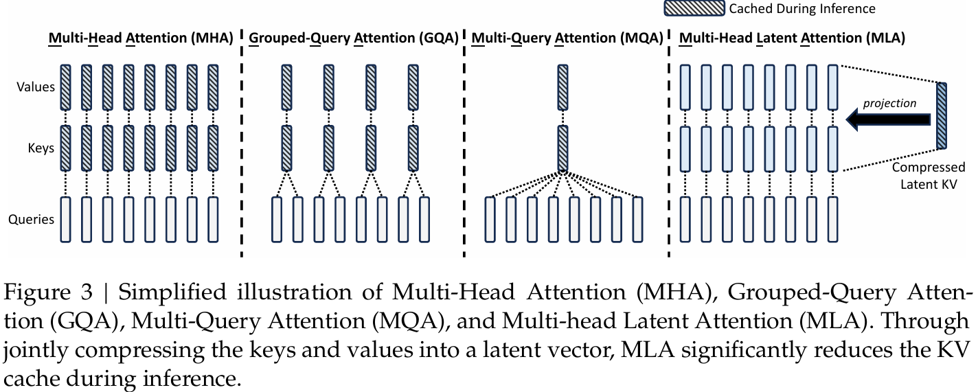
print(output.shape)  # 输出: torch.Size([16, 10, 512])

4. 分组查询注意力（Grouped-Query Attention, GQA）​​

• ​​原理​​：折中方案，将查询头分组，每组共享键和值头（介于MHA和MQA之间）。
• ​​特点​​：平衡计算效率和模型性能。
• ​​应用​​：大模型推理优化（如Llama 2的70B版本）。

import torch
import torch.nn as nn
import torch.nn.functional as F


class GroupedQueryAttention(nn.Module):
    def __init__(self, dim, n_head, n_group=2, dropout=0.1):
        super(GroupedQueryAttention, self).__init__()
        self.dim = dim
        self.head_dim = dim // n_head
        self.n_head = n_head
        self.n_group = n_group
        assert n_head % n_group == 0, "n_head must be divisible by n_group"
        assert self.dim == self.head_dim * n_head
        
        # 分组参数
        self.heads_per_group = n_head // n_group
        
        # 投影层
        self.linear_q = nn.Linear(dim, dim)  # 每个头独立的Q
        self.linear_k = nn.ModuleList([nn.Linear(dim, self.head_dim * self.heads_per_group) for _ in range(n_group)])
        self.linear_v = nn.ModuleList([nn.Linear(dim, self.head_dim * self.heads_per_group) for _ in range(n_group)])
        
        self.dropout = nn.Dropout(dropout)
        self.fc_out = nn.Linear(dim, dim)

    def forward(self, x, mask=None):
        b, t, d = x.size()
        
        # 投影Q (和MHA一样)
        Q = self.linear_q(x).view(b, t, self.n_head, self.head_dim).transpose(1, 2)  # [b, h, t, d_h]
        
        # 分组处理K和V
        K_list, V_list = [], []
        for g in range(self.n_group):
            # 获取当前组的头范围
            start = g * self.heads_per_group
            end = (g + 1) * self.heads_per_group
            
            # 投影当前组的K和V
            K_g = self.linear_k[g](x).view(b, t, self.heads_per_group, self.head_dim).transpose(1, 2)  # [b, h_g, t, d_h]
            V_g = self.linear_v[g](x).view(b, t, self.heads_per_group, self.head_dim).transpose(1, 2)  # [b, h_g, t, d_h]
            
            K_list.append(K_g)
            V_list.append(V_g)
        
        K = torch.cat(K_list, dim=1)  # [b, h, t, d_h]
        V = torch.cat(V_list, dim=1)  # [b, h, t, d_h]
        
        # 注意力计算
        score = torch.matmul(Q, K.transpose(2, 3)) / torch.sqrt(torch.tensor(self.head_dim, dtype=torch.float32))
        
        if mask is not None:
            mask = mask.unsqueeze(1)  # 添加头维度
            score = score.masked_fill(mask == 0, -1e9)
        
        score = F.softmax(score, dim=-1)
        if self.dropout is not None:
            score = self.dropout(score)
        
        output = torch.matmul(score, V).transpose(1, 2).contiguous().view(b, t, d)
        output = self.fc_out(output)
        return output

def generate_mask(len_seq):
    """生成下三角掩码矩阵（用于Decoder的自回归掩码）"""
    return torch.tril(torch.ones(len_seq, len_seq)).bool()

# 测试代码
batch_size, num_heads, seq_len, embed_dim = 16, 8, 10, 512
x = torch.randn(batch_size, seq_len, embed_dim)
mask = generate_mask(seq_len).unsqueeze(0).expand(batch_size, seq_len, seq_len)
gqa = GroupedQueryAttention(embed_dim, num_heads)
print("GQA output:", gqa(x, mask).shape)  # [16, 10, 512]

5. 多查询注意力（Multi-Query Attention, MQA）​

• ​​原理​​：多个查询头（Q）共享同一组键（K）和值（V）头，减少计算量。
• ​​特点​​：牺牲部分表达能力以提升推理速度。
• ​​应用​​：资源受限场景（如边缘设备部署的轻量级模型）。

import torch
import torch.nn as nn
import torch.nn.functional as F
class MultiQueryAttention(nn.Module):
    def __init__(self, dim, n_head, dropout=0.1):
        super(MultiQueryAttention, self).__init__()
        self.dim = dim
        self.head_dim = dim // n_head
        self.n_head = n_head
        assert self.dim == self.head_dim * n_head
        
        # 共享的K和V投影（MQA核心）
        self.linear_q = nn.Linear(dim, dim)  # 每个头独立的Q
        self.linear_k = nn.Linear(dim, self.head_dim)  # 共享的K
        self.linear_v = nn.Linear(dim, self.head_dim)  # 共享的V
        self.dropout = nn.Dropout(dropout)
        self.fc_out = nn.Linear(dim, dim)

    def forward(self, x, mask=None):
        b, t, d = x.size()
        # 投影Q/K/V
        Q = self.linear_q(x).view(b, t, self.n_head, self.head_dim).transpose(1, 2)  # [b, h, t, d_h]
        K = self.linear_k(x).unsqueeze(1).expand(-1, self.n_head, -1, -1)  # [b, h, t, d_h]
        V = self.linear_v(x).unsqueeze(1).expand(-1, self.n_head, -1, -1)  # [b, h, t, d_h]
        
        # Scaled dot-product attention
        score = torch.matmul(Q, K.transpose(2, 3)) / torch.sqrt(torch.tensor(self.head_dim, dtype=torch.float32))
        if mask is not None:
            mask = mask.unsqueeze(1)  # 添加头维度
            score = score.masked_fill(mask == 0, -1e9)
        
        score = F.softmax(score, dim=-1)
        if self.dropout is not None:
            score = self.dropout(score)
        
        output = torch.matmul(score, V).transpose(1, 2).contiguous().view(b, t, d)
        output = self.fc_out(output)
        return output
def generate_mask(len_seq):
    """生成下三角掩码矩阵（用于Decoder的自回归掩码）"""
    return torch.tril(torch.ones(len_seq, len_seq)).bool()

# 测试代码
batch_size, num_heads, seq_len, embed_dim = 16, 8, 10, 512
x = torch.randn(batch_size, seq_len, embed_dim)
mask = generate_mask(seq_len).unsqueeze(0).expand(batch_size, seq_len, seq_len)
mqa = MultiQueryAttention(embed_dim, num_heads)
print("MQA output:", mqa(x, mask).shape)  # [16, 10, 512]

6. 多层注意力（Multi-Head Latent Attention, MLA）​

• ​​原理​​：通过低秩矩阵将KV Cache压缩为潜在问量，显者降低了KV Cache缓存占用和计算成本，提高了推理速度和吞吐量。（deepseek v2）

import torch
import torch.nn as nn
import torch.nn.functional as F

class MultiHeadLatentAttention(nn.Module):
    def __init__(self, input_dim, latent_dim, n_head, dropout=0.1):
        """
        Args:
            input_dim: Dimension of input features
            latent_dim: Dimension of latent space
            n_head: Number of attention heads
            dropout: Dropout probability
        """
        super(MultiHeadLatentAttention, self).__init__()
        self.input_dim = input_dim
        self.latent_dim = latent_dim
        self.n_head = n_head
        self.head_dim = latent_dim // n_head
        
        assert self.latent_dim == self.head_dim * n_head, "latent_dim must be divisible by n_head"
        
        # Projections from input space to latent space
        self.linear_q = nn.Linear(input_dim, latent_dim)
        self.linear_k = nn.Linear(input_dim, latent_dim)
        self.linear_v = nn.Linear(input_dim, latent_dim)
        
        # Latent space projections
        self.latent_proj_q = nn.Linear(latent_dim, latent_dim)
        self.latent_proj_k = nn.Linear(latent_dim, latent_dim)
        
        self.dropout = nn.Dropout(dropout)
        self.fc_out = nn.Linear(latent_dim, input_dim)  # Project back to input dimension
        
    def forward(self, x, mask=None):
        """
        Args:
            x: Input tensor of shape [batch_size, seq_len, input_dim]
            mask: Optional mask tensor of shape [batch_size, seq_len, seq_len]
            
        Returns:
            Output tensor of shape [batch_size, seq_len, input_dim]
        """
        b, t, d = x.size()
        
        # Project input to latent space
        Q = self.linear_q(x)  # [b, t, latent_dim]
        K = self.linear_k(x)  # [b, t, latent_dim]
        V = self.linear_v(x)  # [b, t, latent_dim]
        
        # Further project queries and keys in latent space
        Q_latent = self.latent_proj_q(Q)  # [b, t, latent_dim]
        K_latent = self.latent_proj_k(K)  # [b, t, latent_dim]
        
        # Reshape for multi-head attention
        Q_latent = Q_latent.view(b, t, self.n_head, self.head_dim).transpose(1, 2)  # [b, n_head, t, head_dim]
        K_latent = K_latent.view(b, t, self.n_head, self.head_dim).transpose(1, 2)  # [b, n_head, t, head_dim]
        V = V.view(b, t, self.n_head, self.head_dim).transpose(1, 2)  # [b, n_head, t, head_dim]
        
        # Scaled dot-product attention in latent space
        scores = torch.matmul(Q_latent, K_latent.transpose(-2, -1)) / torch.sqrt(torch.tensor(self.head_dim, dtype=torch.float32))
        
        # Apply mask if provided
        if mask is not None:
            mask = mask.unsqueeze(1)  # Add head dimension
            scores = scores.masked_fill(mask == 0, -1e9)
        
        # Softmax and dropout
        attn_weights = F.softmax(scores, dim=-1)
        if self.dropout is not None:
            attn_weights = self.dropout(attn_weights)
        
        # Apply attention to values
        output = torch.matmul(attn_weights, V)  # [b, n_head, t, head_dim]
        
        # Combine heads and project back to input dimension
        output = output.transpose(1, 2).contiguous().view(b, t, self.latent_dim)
        output = self.fc_out(output)  # [b, t, input_dim]
        
        return output

def generate_mask(len_seq):
    """Generate lower triangular mask matrix (for autoregressive masking in decoder)"""
    return torch.tril(torch.ones(len_seq, len_seq)).bool()

# 使用案例
num_heads, input_dim, latent_dim = 8, 512, 256
model = MultiHeadLatentAttention(input_dim, latent_dim, num_heads)
x = torch.randn(16, 10, input_dim)  # Input shape: [batch_size, seq_len, input_dim]
mask = generate_mask(10).unsqueeze(0).expand(16, 10, 10)
output = model(x, mask)
print(output.shape)  # Output: torch.Size([16, 10, 512])

六、位置编码(正余弦PE，ROPE，RPE，ROPE+ 2D RPE)

场景	推荐方法	代表模型
RoPE	目前LLM的主流选择，外推能力强	LLaMA、BaiChuan、ChatGLM、GPT-NeoX
RPE（相对位置编码）	固定长度/局部依赖强（如 BERT、T5、Swin Transformer）	T5、Swin Transformer
RoPE（文本）+ 2D RPE（视觉）	多模态模型（文本+视觉）​​	BLIP-2（Q-Former）、Fuyu-8B
ALiBi/NTK-aware RoPE	长序列推理，长文本优化	BLOOM、CodeLlama、Mistral
LAPR（可学习绝对位置编码）	早期模型，现在逐渐被淘汰； 外推能力差;无法显式建模相对位置关系	GPT-2、原始BERT

1. 绝对位置编码(正余弦位置编码)

• 对于偶数维度（即2*i位置）；对于奇数维度（即2*i+1位置），其中i = d_model // 2。

import torch
import math

def position_encoding(seq_len, d_model):
    # 创建一个空的张量用于存储位置编码
    position = torch.arange(0, seq_len).unsqueeze(1).float()  # [seq_len, 1] --> (10, 1)
    dim = torch.arange(0, d_model // 2).float()  # [d_model // 2]   # (1, 8)
    # 计算位置编码
    encoding = position / (10000 ** (2 * dim / (d_model)))  # [10, 16 // 2]
    # 分别计算sin和cos
    sin_enc, cos_enc = torch.sin(encoding), torch.cos(encoding)  # sin编码, cos编码   
    print(sin_enc.shape)
    # 将sin和cos交替插入，得到完整的编码(sin值放到偶数位置, cos值放到奇数位置)
    encoding = torch.zeros(seq_len, d_model)  # [seq_len, d_model]
    encoding[:, 0::2], encoding[:, 1::2] = sin_enc, cos_enc
    return encoding

seq_len, d_model = 10, 16  # 序列长度, 嵌入维度
encoding = sinusoidal_position_encoding(seq_len, d_model)
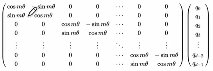
print("Sin_Cos PE:\n", encoding)

2. 旋转位置编码（ROPE）

• Reference

        (1) 大模型Embedding整明白了！RoPE位置编码真简单！_哔哩哔哩_bilibili

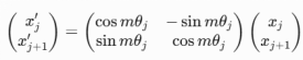
        (2) 十分钟读懂旋转编码（RoPE）

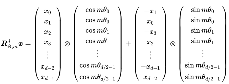
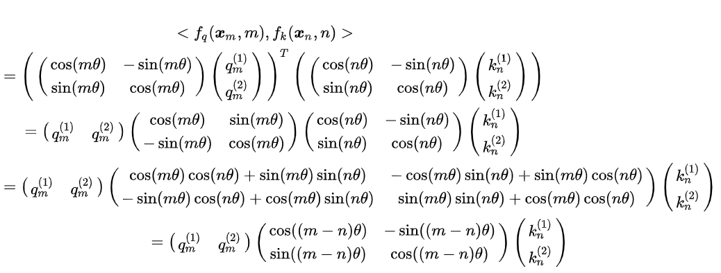
• 核心思想：将位置信息编码为旋转矩阵，作用于查询(Query)和键(Key)的注意力计算中，隐式融合绝对位置(θj = 10000−2j/d)与相对位置(m-n)的双重特性。ROPE 位置编码通过将一个向量旋转某个角度，为其赋予位置信息。对Query和Key的每个token维度对 (xi, xi+1) 应用旋转矩阵，其中θi = 10000−2i/d（频率递减）。
• 优点：
  • 外推性强:支持超长序列推理(如LLaMA-2支持4k→16k扩展)；
  • 远程衰减:通过波长设计自动衰减远发离依赖；
  • 数学等价:通过旋转操作实现相对位置偏移的数学等价性。
• 使用场景：
  • 长文本生成(如Qwen系列模型)，需处理超长上下文(如32Ktoken以上)；
  • 多模态任务(如图文对齐)，需灵活适配不同态的序列长度。
• 关键公式：

### 手撕ROPE
import torch
import torch.nn as nn
import numpy as np
np.random.seed(42)
torch.manual_seed(42)


class RotaryEmbedding(nn.Module):
    def __init__(self, d_model, num_heads, base=10000, max_len=512):
        super().__init__()
        self.head_dim = d_model // num_heads
        half_dim = self.head_dim // 2
        pos = torch.arange(max_len).float()
        freqs = 1.0 / (base ** (2 * torch.arange(half_dim).float() / self.head_dim))
        angles = torch.einsum("i,j->ij", pos, freqs)  # m*θ  [max_len, half_dim]
        sin = torch.sin(angles).repeat_interleave(2, -1)   # sin(m*θ)
        cos = torch.cos(angles).repeat_interleave(2, -1)   # cos(m*θ)
        self.register_buffer("cos", cos[None, :, :])  # [1, max_len, head_dim]
        self.register_buffer("sin", sin[None, :, :])  # [1, max_len, head_dim]

    def forward(self, q):  # q: [B, T, D]
        B, T, D = q.shape
        q = q.view(B, T, -1, self.head_dim).transpose(1, 2)  # [B, H, T, D/H]
        cos = self.cos[:, :T, :].unsqueeze(1)  # [1, 1, T, D/H]
        sin = self.sin[:, :T, :].unsqueeze(1)
        # 把 q（形状 [B, H, T, D/H]）分成两个子张量：
        # q1: 取偶数维度（即第 0、2、4…），q2: 取奇数维度（即第 1、3、5…）
        q1, q2 = q[..., ::2], q[..., 1::2]  
        q_rot = torch.stack([q1 * cos[..., ::2] - q2 * sin[..., ::2],
                             q1 * sin[..., ::2] + q2 * cos[..., ::2]], dim=-1)
        return q_rot.flatten(-2, -1)  # [B, H, T, (D/H)/2, 2]--> [B, H, T, D/H]

# 示例调用
bs, num_heads, T, d_model = 4, 8, 128, 512
q = torch.randn(bs, seq_len, d_model)
rope = RotaryEmbedding(d_model, num_heads)
q_rope = rope(q)
q_rope.shape   # [4, 8, 128, 64]

• ROPE V.S. 绝对PE(正余弦编码)

特性​​	RoPE​​	绝对PE（LAPR）​​
位置信息注入	通过旋转融入Q/K计算（动态）	直接加到输入上（静态）
相对位置感知	✅ 自动编码相对距离	❌ 需模型自行学习
外推能力	✅ 支持任意长度（旋转矩阵普适）	❌ 超出训练长度时失效
计算效率	O(1)（无需存储位置矩阵）	O(L)（需存储位置嵌入）
适用场景​​	大模型、长文本	固定长度任务（如BERT）

• 为什么理论上可以无限外推
  • 数学原理：RoPE的旋转矩阵性质保证：对于任意位置差 k=m−n，旋转角度 θj​k 始终有效，与 m,n 的绝对值无关。
  • 频率衰减设计：高频（小 j）编码局部信息，低频（大 j）编码全局信息，确保长程依赖仍能被捕捉。
  • 工程表现：即使推理时输入远超训练长度（如训练4k，推理32k），RoPE无需调整仍能保持性能（如LLaMA-2的上下文扩展）。
• 无限长输入的原因与解决方案：原因——注意力计算复杂度，原始自注意力的 O(L2) 计算成本；训练数据偏差，长文本的稀疏性使模型未充分学习远距离依赖。解决方案——稀疏注意力，如Longformer的滑动窗口；外推优化，NTK-aware RoPE：动态调整频率基θj​（如CodeLlama）；线性插值，将位置索引 m 压缩为 m/α（α 为缩放因子）。
• 怎么控制image token的长度
  • Patch合并：ViT将图像分割为 N×N patches（如14×14=196），通过卷积步长或池化减少token数。
  • 可学习查询压缩：Q-Former用少量可学习query（如32个）通过交叉注意力聚合视觉特征。
  • Perceiver Resampler：使用固定数量的latent token（如64）压缩原始视觉token。

七、Decoder解码

策略​​	优点​​	缺点​​	适用场景​​
Greedy Search	简单高效	缺乏多样性	确定性任务（如机器翻译）
Beam Search	更全局化的决策	计算开销大，可能生成通用文本，改进用n-gram策略。	文本摘要、翻译
Temperature Sampling	灵活控制多样性	需调参 T	开放域生成（如对话）
Top-k Sampling	过滤低质量词	k 固定，可能不适应所有上下文	通用文本生成
Top-p Sampling	动态候选词数量，更鲁棒	需调参 p	创意写作、故事生成

1. Greedy Search

• ​​原理​​：每一步选择当前概率最高的词，即 argmax(P(w|context))；
• ​​特点​​：计算高效，但可能陷入重复或局部最优；缺乏多样性，生成结果可能过于保守。

def greedy_search(logits):
    return torch.argmax(logits, dim=-1)
# 示例
logits = torch.tensor([[0.1, 0.5, 0.4]])
print(greedy_search(logits))  # 输出: tensor([1])

2. Beam Search

• 原理​​：保留Top-K（beam_width）个候选序列，每一步扩展这些序列并保留总概率最高的K个；
• ​​特点​​：比贪心搜索更全局化，但可能生成过于通用的文本（使用n-gram策略改进）；超参数 beam_width 影响效果和计算开销。

def beam_search(logits, beam_width=2):
    probs, indices = torch.topk(logits.softmax(dim=-1), beam_width, dim=-1)
    return indices, probs
# 示例
logits = torch.tensor([[0.1, 0.5, 0.4]])
indices, probs = beam_search(logits)
print(indices)  # 输出: tensor([[1, 2]])

3. Temperature Sampling

• ​​原理​​：通过温度参数 T 调整概率分布：
  • T=1：原始分布；
  • T>1：平滑分布（更多多样性）；
  • T<1：尖锐分布（更确定性）；
  • P(w) = exp(logits/T) / sum(exp(logits/T))

def temperature_sampling(logits, temperature=1.0):
    probs = torch.softmax(logits / temperature, dim=-1)
    return torch.multinomial(probs, num_samples=1)    # 概率分布采样
# 示例
logits = torch.tensor([[1.0, 2.0, 3.0]])
print(temperature_sampling(logits, temperature=0.5))  # 可能输出: tensor([2])

4. Top-k Sampling（手撕）

• 原理：仅从概率最高的前 k 个词中采样，过滤低概率词；
• 特点：平衡多样性与质量，但 k 是固定值，可能在某些上下文下不合适。

def top_k_sampling(logits, k=2):
    values, indices = torch.topk(logits, k)
    probs = torch.softmax(values, dim=-1)
    return indices[torch.multinomial(probs, 1)]
# 示例
logits = torch.tensor([[1.0, 2.0, 3.0, 4.0]])
print(top_k_sampling(logits, k=2))  # 可能输出: tensor([3])

5. Top-p Sampling（手撕）

• 原理：从累积概率超过阈值 p 的最小词集合中采样;
• 特点：动态调整候选词数量，适应不同上下文。

def top_p_sampling(logits, p=0.9):
    probs = torch.softmax(logits, dim=-1)
    sorted_probs, sorted_indices = torch.sort(probs, descending=True)
    cum_probs = torch.cumsum(sorted_probs, dim=-1)
    mask = cum_probs <= p
    mask = torch.cat([torch.ones_like(mask[:1]), mask[:-1]], dim=0)
    filtered_probs = sorted_probs * mask
    sampled_idx = torch.multinomial(filtered_probs, 1)
    return sorted_indices[sampled_idx]
# 示例
logits = torch.tensor([[0.1, 0.3, 0.2, 0.4]])
print(top_p_sampling(logits, p=0.8))  # 可能输出: tensor([3])

八、NLP、CV、AIGC、MLLMs经典算法

(写不动了，后面再填坑吧......)

1. NLP

        rnn, lstm, attention, bert, gpt, transformer；

2. CV

        cnn, vit, resnet, clip, blip, yolo系列, fastcnn, detr, inception, sam, dino；

3. AIGC

        VAE系列, GAN系列，Text-Guided系列, SD系列-ddpm/ddim/ldm/repaint-fastpaint论文，SD优劣&常见的采样方式（ddim,dpm++,lcm,turbo）&原理&loss函数，sdxl相对sd的改进方式；

4. MLLMs

        CLIP，SigLIP，EVA-CLIP，ALBEF，BLIP，BLIP2，Instruct-BLIP，Flamingo，MiniCPM-V，LlaVA，CogVLM，Qwen-VL系列，InternVL系列，Deepseek-多模系列；

        在“ 多模态学习路线（3）—— MLLMs主流模型 ”里会更新 & 详细介绍。