03假设检验续

一、非正态分布

1.chi-square 检验

研究背景

遗传学的一个基本问题是确定实验确定的数据是否符合理论预期的结果

如何判断观察到的一组后代数量是否是给定的底层简单比率的合法结果？

卡方检验适用的环境

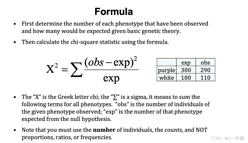
卡方检验是一种“拟合优度”检验：它回答了观察到的数据与预期的符合程度的问题。

chisq.test (c(315,101,108,32), p = c(9/16,3/16,3/16,1/16))

#没太明白这里的实际意思。

如何定义接近这是个问题，chi-square来定义接近的好方法。

chi-square像是组方，卡方分布。

1-pchisq(1.333,df=1) # 0.24
# 卡方分布的累积概率密度函数，这算的是大于的情况
#（为什么自由度为1）

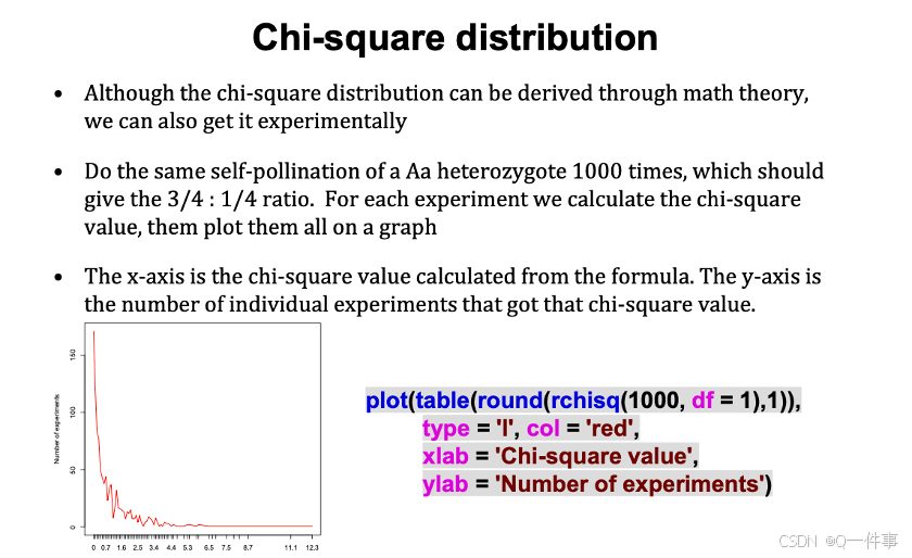
对 Aa 杂合子进行 1000 次相同的自花授粉，应产生 3/4 : 1/4 的比例。对于每个实验，我们计算卡方值，然后将它们全部绘制在图表上。

plot(table(round(rchisq(1000, df = 1),1)),
type = 'l', col = 'red',
xlab = 'Chi-square value',
ylab = 'Number of experiments')

这上面每个函数的每个值需要弄清楚。

plot(table(round(rchisq(1000, df = 1),1)),
type = 'l', col = 'red',
xlab = 'Chi-square value',
ylab = 'Number of experiments')
# 随机产生，自由度为1度卡方分布，所有差距平方之和

当为一个条形图时，这个情况更加的显著。

hist ( rchisq (1000, df =1),
nclass=30 )

绘制卡方分布，不同自由度下，数量与分布的情况。

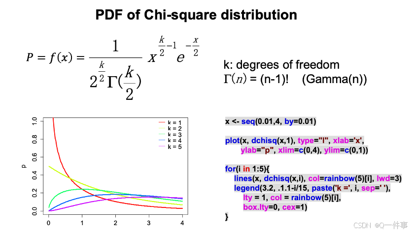
x <- seq(0.01,4, by=0.01)
plot(x, dchisq(x,1), type="l", xlab='x',
ylab="p", xlim=c(0,4), ylim=c(0,1))
for(i in 1:5){
lines(x, dchisq(x,i), col=rainbow(5)[i], lwd=3)
legend(3.2, 1.1-i/15, paste('k =', i, sep=' '),
lty = 1, col = rainbow(5)[i],
box.lty=0, cex=1)
}
# 这个算出了概率密度函数，1-5

2.正确性分析

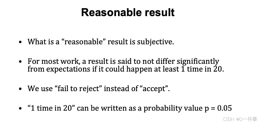
对于结果的正确性，我们从来不能判断，但是我只能说这个结果想不想正确的结果。

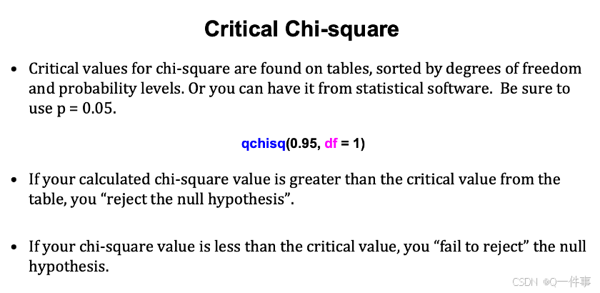
影响卡方分布的只有一个值，自由度等于类别减去1（自由度是类别数减去1）

qchisq(0.95, df = 1) #得到临界值
### 

当大于计算出来的统计量可以拒绝原假设，然后再进行分析。

chi square test

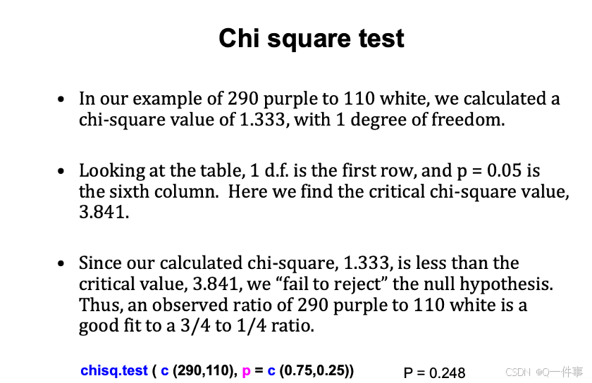
比较他们之间的相似性。

chisq.test ( c (290,110), p = c (0.75,0.25)) 

chisq.test(c(315, 101,108,32), p= c(9/16, 3/16, 3/16, 1/16))

qchisq(0.95, df = 1)#得到临界值
### ？？这个值没太明白。

x <- seq(0.01,10, by=0.01)
plot(x, dchisq(x,3), type="l", xlab='x',
ylab="p", xlim=c(0,10), ylim=c(0,.3))
abline(0,0)
abline(v=0.47, lwd=3) # Mendel’s result
abline(v=qchisq(.95, 3), lwd=3, col ="red") # 5%

# 什么时候拒绝这个假定，可以计算其统计量。

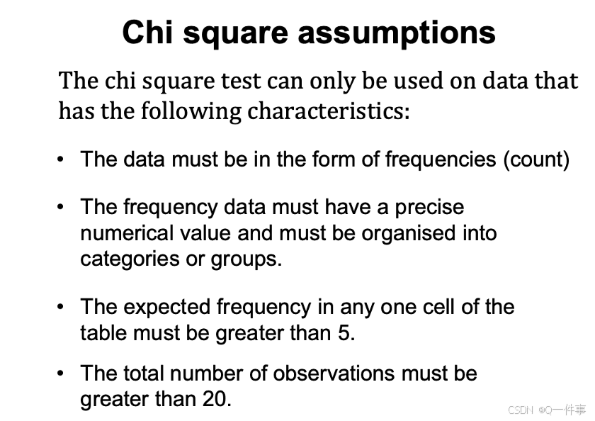
卡方检验的假定

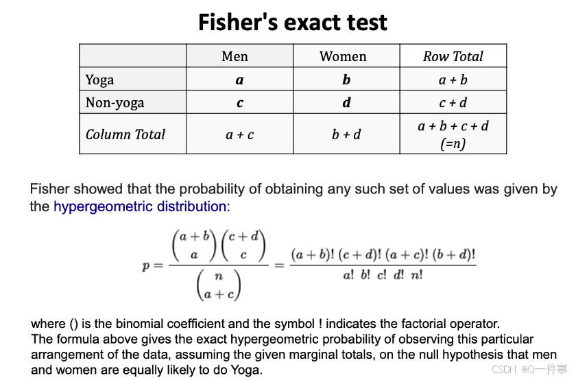
2.Fisher的精确性检验

样本量太少的话，用fisher的精确性检验。非比例的结果

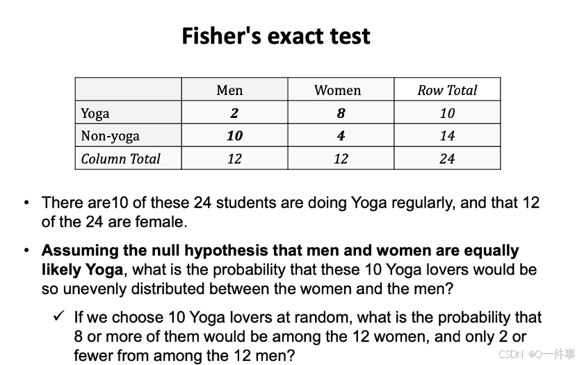
fisher能解决这个结果，和结果更靠外的结果。fisher能解决更靠外的结果。

TeaTasting <- matrix(c(8, 2, 3, 7), nrow = 2,
dimnames = list(Guess = c("Milk", "Tea"),
Truth = c("Milk", "Tea")))
fisher.test(TeaTasting, alternative = "greater")

4✖️4的结果也能解释

选择正确性

TeaTasting <- matrix(c(8, 2, 3, 7), nrow = 2,
dimnames = list(Guess = c("Milk", "Tea"),
Truth = c("Milk", "Tea")))
fisher.test(TeaTasting, alternative = "greater")

工作满意度的分析

## A 4 x 4 table Agresti (2002, p. 57) Job Satisfaction
Job <- matrix(c(1,2,1,0, 3,3,6,1, 10,10,14,9, 6,7,12,11), 4, 4,
dimnames = list(income = c("< 15k", "15-25k", "25-40k", "> 40k"),
satisfaction = c("VeryD",
"LittleD",
"ModerateS",
"VeryS")))
fisher.test(Job)
fisher.test(Job, simulate.p.value = TRUE, B = 1e5)#这里是fisher检验

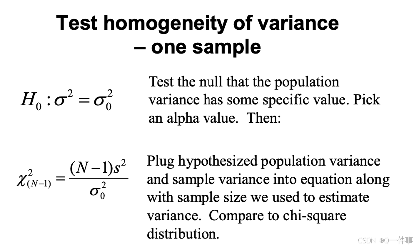
3.测试方差齐性

测试方差齐性。

var.test() # 需要满足很多的条件
bartlett.test() # 适用于正态分布
fligner.test() # 计算x，y变量不一样的情况
# 上面备注的参考文献：https://blog.youkuaiyun.com/dataxc/article/details/115833293

# 多样本方差比较的Bartlett检验
# 参考：https://www.cnblogs.com/ayueme/articles/16844527.html

卡方检验是单位的检验

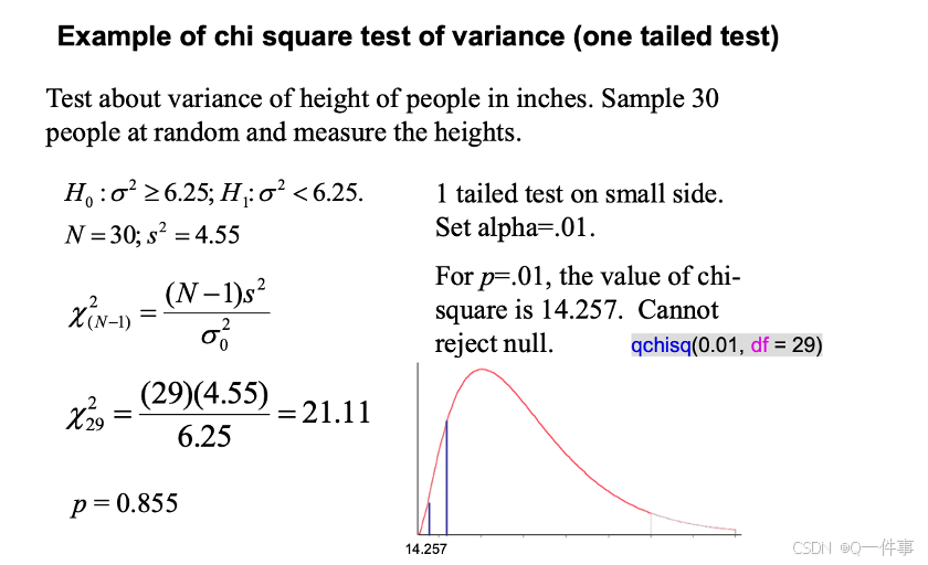
qchisq(0.01, df = 29)

计算两个独立变量的方差齐性，是比较那个方差是否有差别，一般来说，方差的大小的容忍度还是很大的。

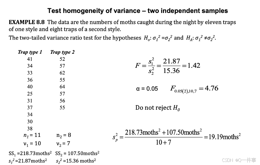
这块是检验两个方差是否存在显著性差异，最后算出是差不多五倍，没有存在显著性差异。

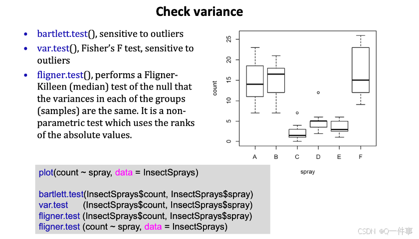
（如果这个有很多个组分我们要如计算呢？）

plot(count ~ spray, data = InsectSprays)
bartlett.test(InsectSprays$count, InsectSprays$spray)

# t检验 这个是报错的
var.test(InsectSprays$count, InsectSprays$spray)

# F检验 
fligner.test (InsectSprays$count, InsectSprays$spray)
fligner.test (count ~ spray, data = InsectSprays)

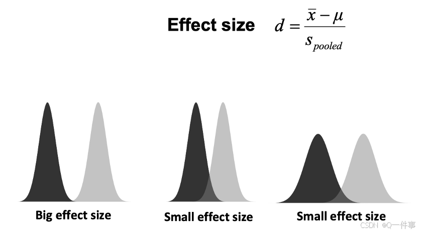
二、Effect size

p值越小，显著性越大。

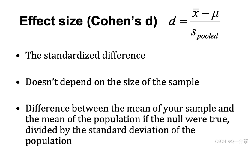
effect.size <- function(data.1, data.2){
d <- (mean(data.1) - mean(data.2))/
sqrt(((length(data.1) - 1) * var(data.1) +
(length(data.2) - 1) * var(data.2))/
(length(data.1) + length(data.2)-2))
names(d) <- "effect size d"
return(d)
}
effect.size(rnorm(30),rnorm(50,2,1))

plot.design(breaks ~ wool + tension, data = warpbreaks)

effect能说明什么呢？

positive是推翻原假设的结果

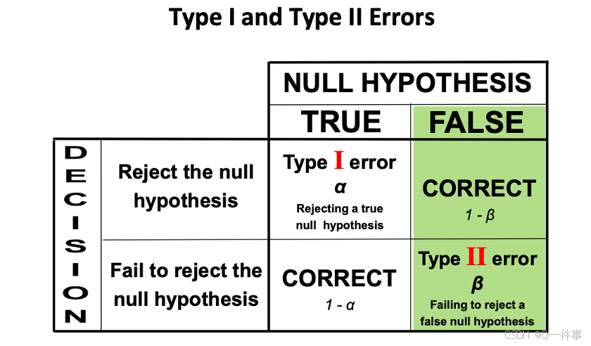
三、Power of test

如何计算第二类错误。

原假设算临界值，临界值要算第二个来算。

n = 30 # sample size
sigma = 120 # population standard deviation
sem = sigma/sqrt(n); sem # standard error
alpha = .05 # significance level
mu0 = 10000 # hypothetical lower bound
q = qnorm(alpha, mean=mu0, sd=sem)

q

mu = 9950 # assumed actual mean
pnorm(q, mean=mu, sd=sem, lower.tail=FALSE)

power分析

power.t.test (n = 20, delta = 1.5, sd = 2, sig.level = 0.05,
type = "one.sample"
, alternative = "two.sided"
, strict = TRUE)

library (pwr)
pwr.t2n.test (n1 = 30, n2 = 50,
d = -.5, sig.level = 0.05,
alternative = "less")

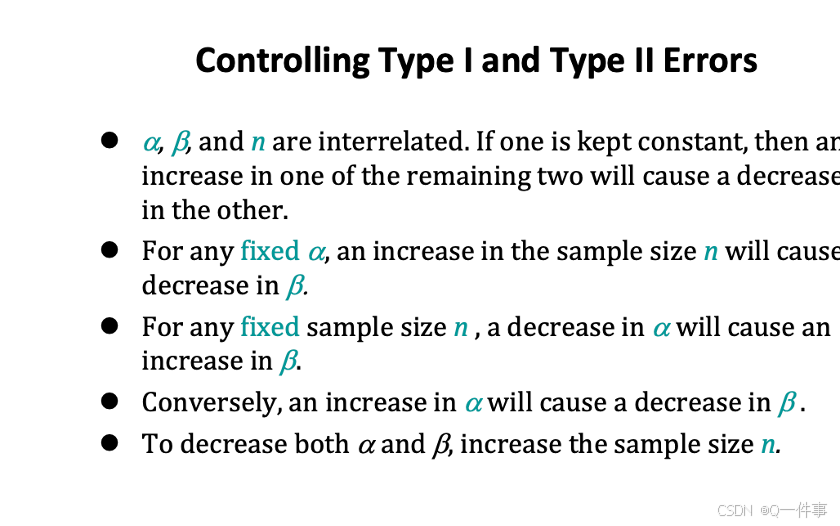
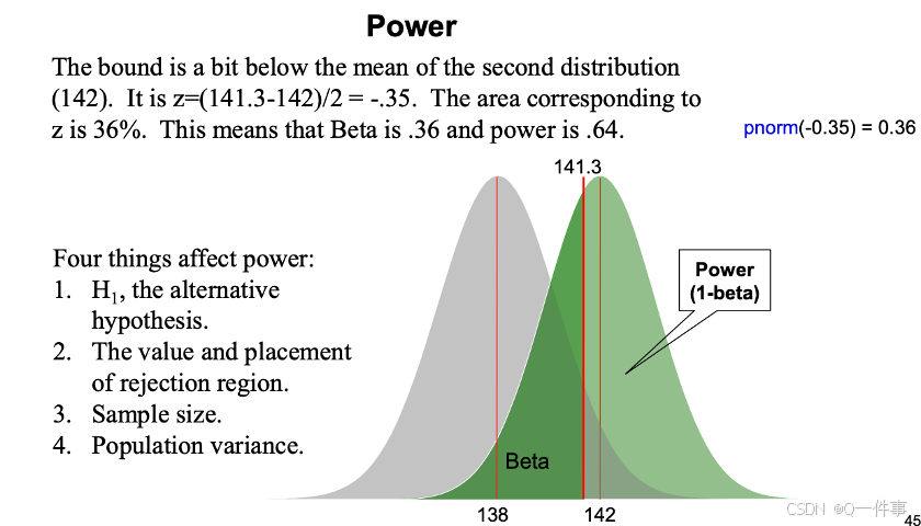
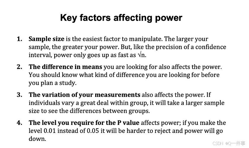
影响power的因素。

pnorm(-0.57) # 0.28
pt(-0.57, 11) # 0.29

设置错误的水平

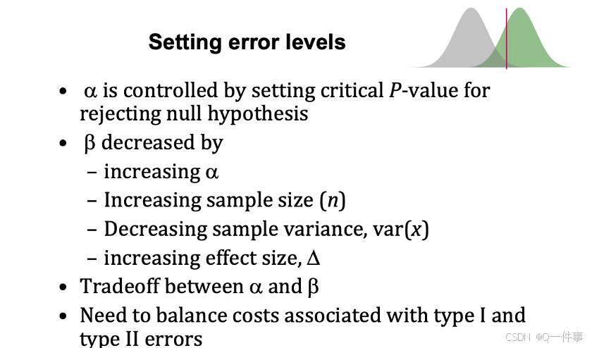
样本量增加会变大

1.如何影响p值

（1）样本真正的差异

（2）样本的数量

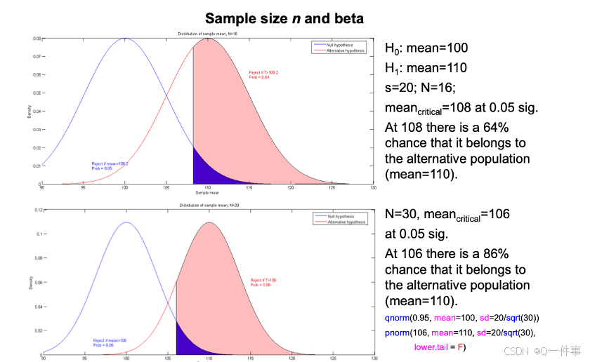
qnorm(0.95, mean = 100, sd = 20/sqrt(30))
pnorm(106,mean =110, sd = 20/sqrt(30), lower.tail = F)

pnorm(108,mean =110, sd = 20/sqrt(30), lower.tail = F)

library(pwr)
# range of correlations
r <- seq(.1,.5,.01)
nr <- length(r)
# power values
p <- seq(.4,.9,.1)
np <- length(p)
# obtain sample sizes
samsize <- array(numeric(nr*np), dim=c(nr,np))
for (i in 1:np){
for (j in 1:nr){
result <- pwr.r.test(n = NULL, r = r[j],
sig.level = .05, power = p[i],
alternative = "two.sided")
samsize[j,i] <- ceiling(result$n)
 }}
samsize

# set up graph
xrange <- range(r)
yrange <- round(range(samsize))
colors <- rainbow(length(p))
plot(xrange, yrange, type="n",
xlab = "Correlation Coefficient (r)",
ylab = "Sample Size (n)" )
# add power curves
for (i in 1:np){
lines(r, samsize[,i],type="l",lwd=2,col=colors[i])
}
# add annotation (grid lines, title, legend)
abline(v=0, h=seq(0,yrange[2],50), lty=2, col="grey89")
abline(h=0, v=seq(xrange[1],xrange[2],.02), lty=2,col="grey89")
title("Sample Size Estimation for Correlation Studies\n
Sig=0.05 (Two-tailed)")
legend("topright"
, title="Power", as.character(p), fill=colors)

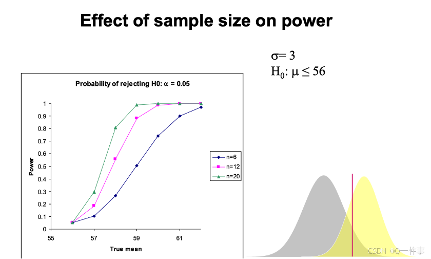
**总结：**当研究的数量越多和研究的真正差距越大（mean和均值差距），它的power值越大。

a <- 6; s <- 2; n <- 20
diff <- qt(0.975, df = n-1)*s/sqrt(n)
left <- a-diff ; right <- a+diff

assumed <- a + 1.5
tleft <- (assumed - right)/(s/sqrt(n)) #1.261
p <- pt(-tleft, df = n-1); p #0.1112583

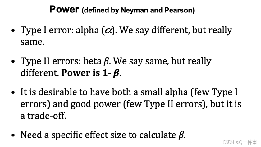
第二类错误是0.2，最大是

事实上，power也可以衡量两个函数之间的差异性。差异性越大实施上越好，又使得第二类错误的前提的概率性降低，事实上也在降低其总体的错误的概率。

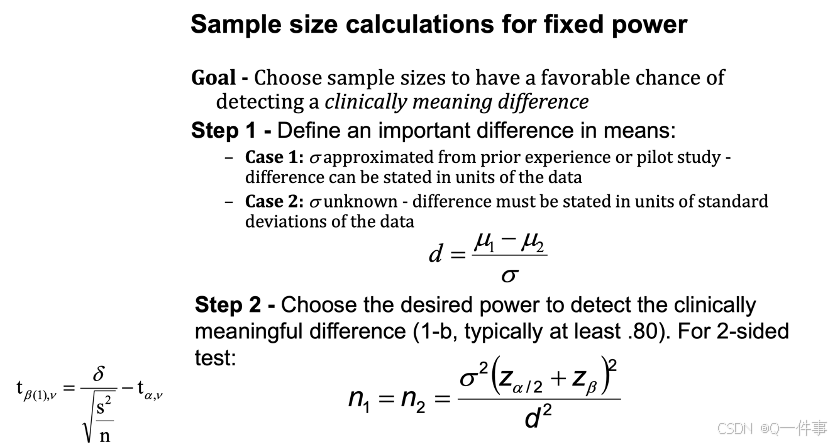
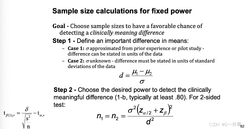
四、Sample size

相关性越大，power越大。这个部分还是挺有意思的。

xrange <- range(r)
yrange <- round(range(samsize))
colors <- rainbow(length(p))
plot(xrange, yrange, type="n",
xlab = "Correlation Coefficient (r)",
ylab = "Sample Size (n)" )
# add power curves
for (i in 1:np){
lines(r, samsize[,i],type="l",lwd=2,col=colors[i])
}
# add annotation (grid lines, title, legend)
abline(v=0, h=seq(0,yrange[2],50), lty=2, col="grey89")
abline(h=0, v=seq(xrange[1],xrange[2],.02), lty=2,col="grey89")
title("Sample Size Estimation for Correlation Studies\n
Sig=0.05 (Two-tailed)")
legend("topright"
, title="Power", as.character(p), fill=colors)

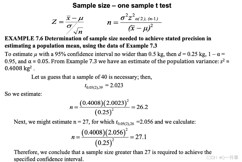
最好样本是30个，最小则是27个。

参考：
https://github.com/Xinhai-Li/Statistics_Courses/tree/master