02假设检验

1.假设检验

差别大不大，大小和影响差别的干扰影响。

有些可能是由于误差上的改变

assumptions 前提条件

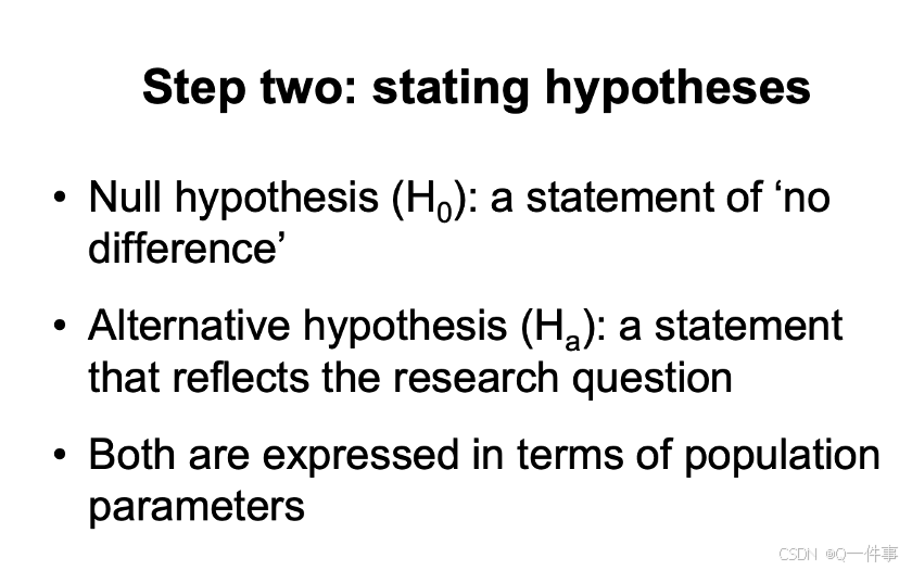
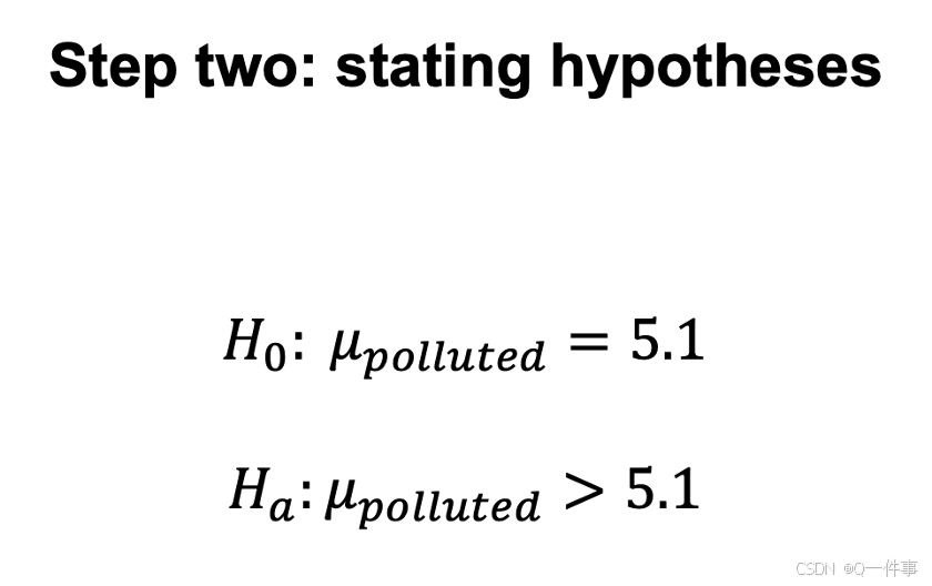
hypothesis 假设

连续变量才能做t检验

hypothesis 这个页面

hist(rbinom(100000, 100, .5), freq = F, main = "",
xlab = 'Number of head', ylab = 'Probability density')

t 检验也称为 Student t 检验，它是一种使用假设检验来评估一个或两个总体均值的工具。t 检验可用于评估某个组是否与已知值有差异（单样本 t 检验），两个组是否彼此有差异（独立双样本 t 检验），或成对测量值中是否存在显著差异（成对或非独立样本 t 检验）。

参考文献：https://www.jmp.com/zh_cn/statistics-knowledge-portal/t-test.html

daily.intake = c(5260,5470,5640,6180,6390,6515,
6805,7515,7515,8230,8770)
mean(daily.intake)
sd(daily.intake)
quantile(daily.intake)
t.test(daily.intake, mu = 7725)

# Nonparametric
wilcox.test(daily.intake, mu = 7725)

# Two samlpes
x1 = rnorm(300, 0, 1)
x2 = sample(0:100, 300, rep = T)
t.test(x1, x2)

# Check normality
plot(x1); hist(x1); qqnorm(x1)
shapiro.test(x1)

假设的整个过程

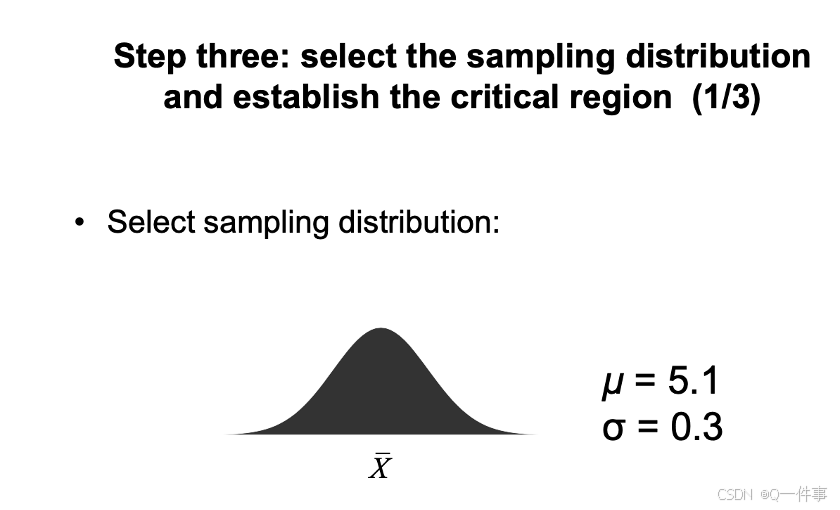
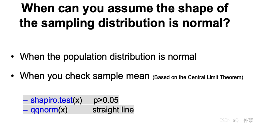
第一步：第一步需要是正态

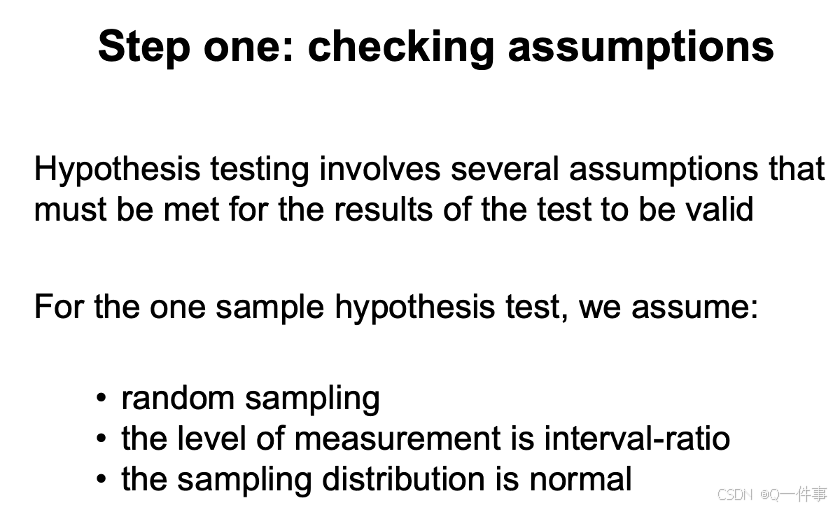
第二步：条件：1.随机分布 2.连续取样 3.样本正态的。

做出两个假设，取样。

判断是否正态1.p值是否小于0.05 2.画图俩分析。

样本量增加会增加其特点，样本量足够大，能够显著性会提高。

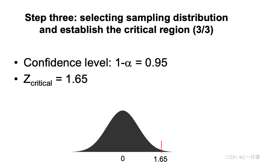
第三步：

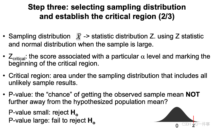
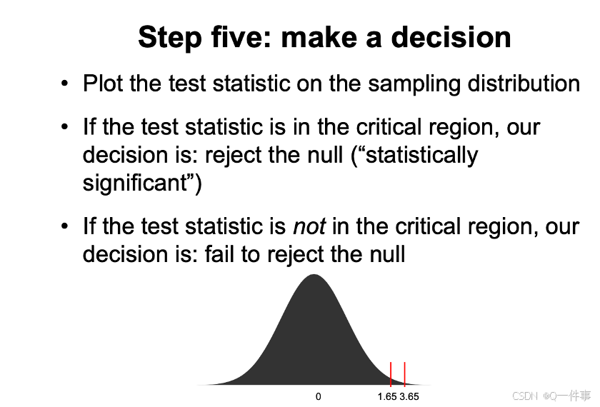
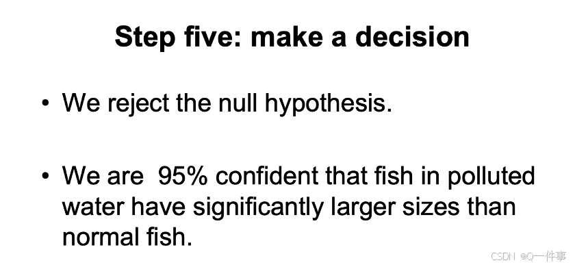
第五步：做出决定。

2.分析回顾

样本量很大

检验正态的分布

（1）如何判断样本是否正态

判断的方法

shapiro.test(x) #p>0.05
qqnorm(x) #straight line

shapiro.test(rnorm(5000, mean = 5, sd = 100))
shapiro.test(runif(30, min = 2, max = 4))

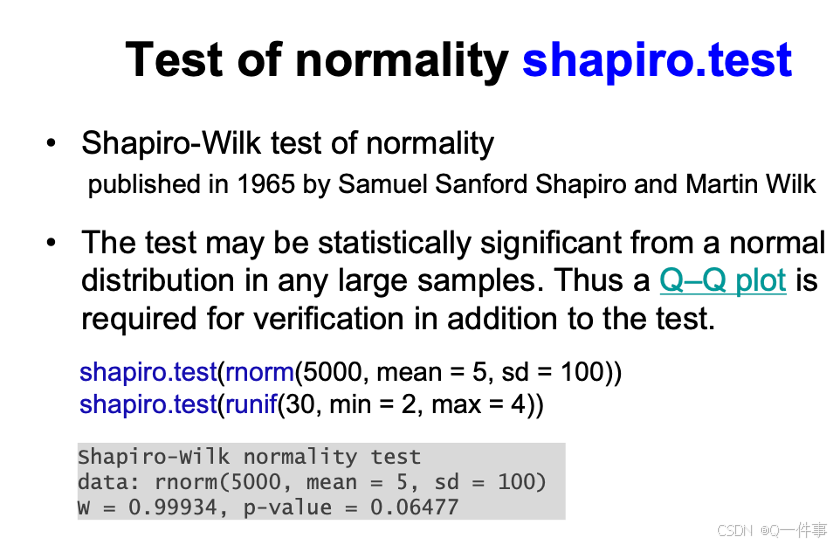
shapiro检验可能在任何大的样本中都显示是正态分布的，因而需要引入QQ图

y <- rnorm(200, sd = 10)
qqnorm(y)
qqline(y, col = 2)

极限中值定律，它的均值是符合正态分布的，这个是可以进行证明的。

# The central limit theorem
# Exponential distribution is a skewed distribution
y <- rexp(100); hist(y, col = 'grey')
# Define a vector with length 200

sample.mean <- numeric(200)
# The mean of 200 samples
for(i in 1:200) sample.mean[i] <- mean(rexp(100))

# A normal distribution appears
hist(sample.mean , col = 'grey')
shapiro.test(sample.mean)

（1）原假设的理解

和样本量无关，是根据图片来看，中间的分布比较多，两边比较少，认为就认为它是正态分布。

原假设必须等于，等于某个值就有个分布，不能大于。大于则分析其原因。分析统计量，最后来计算。

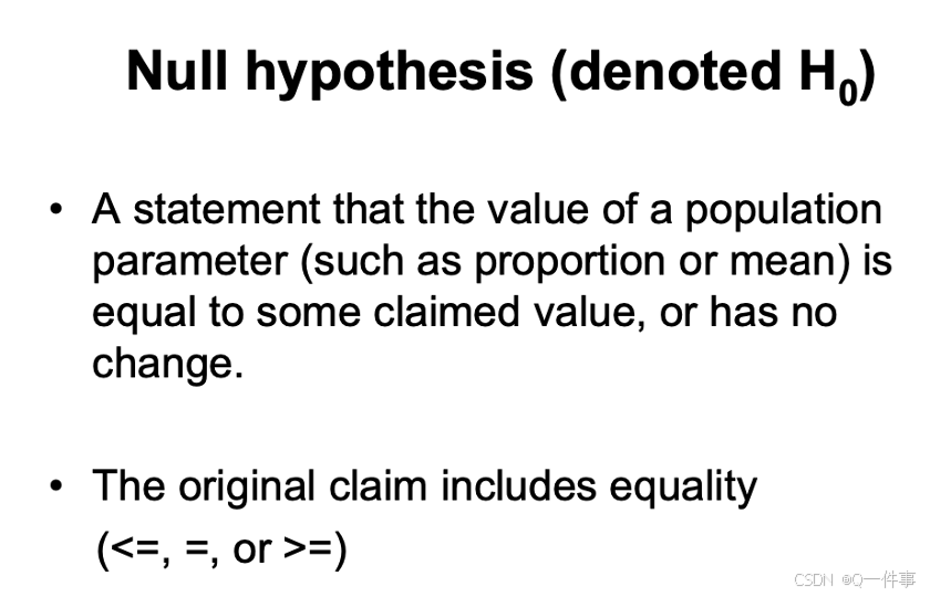
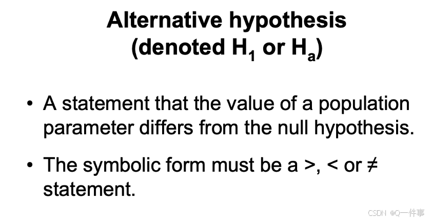
备择假设

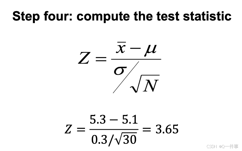
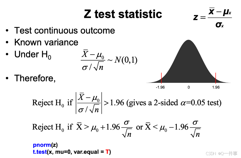
计算统计量

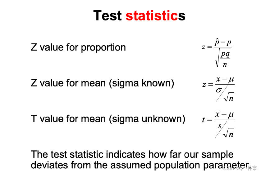
pnorm(z)
t.test(x, mu=0, var.equal = T)

t检验

t.test(x, mu=0, var.equal = F)

自由度相当于样本量。自由度越大。样本量大于30认为是可以正态分布。

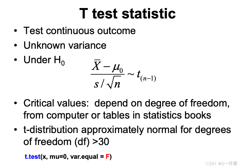
t分布与正态分布相似，t分布扁一点。（样本量少的时候，我们用t分布。）

# Plot a normal distribution and t distributions
x <- seq(-4, 4, len = 1000)
z <- dnorm(x, 0, 1)
plot(x, z, type = 'l', col = 'blue') # the normal curve
segments( 1.96, -0.05, 1.96, 0.1, col = 'brown')
segments(-1.96, -0.05,-1.96, 0.1, col = 'brown')
abline(0,0)
lines(x, dt(x, 15), col = 'green')
lines(x, dt(x, 4), col = 'red')

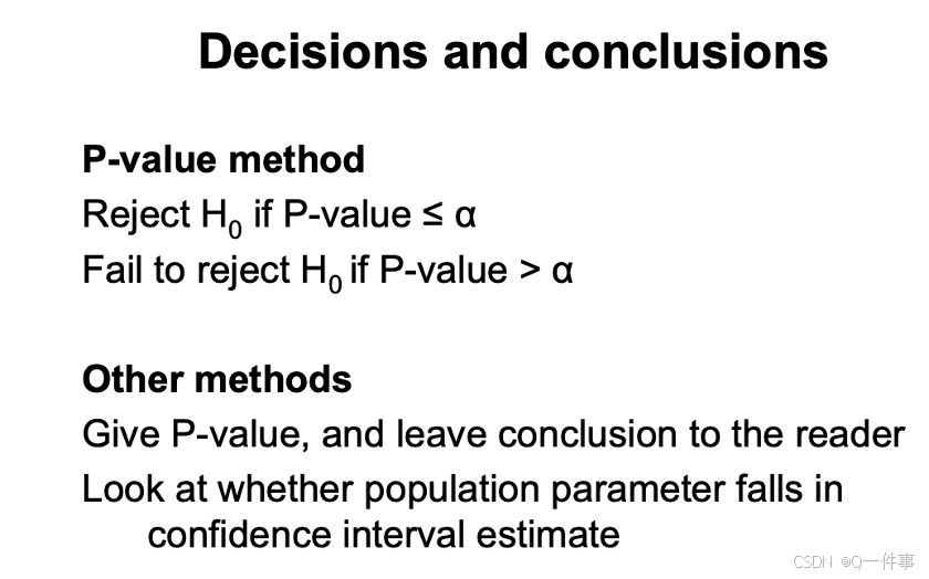
3.陈述假设检验

p值的情况

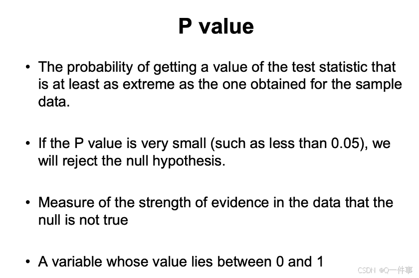
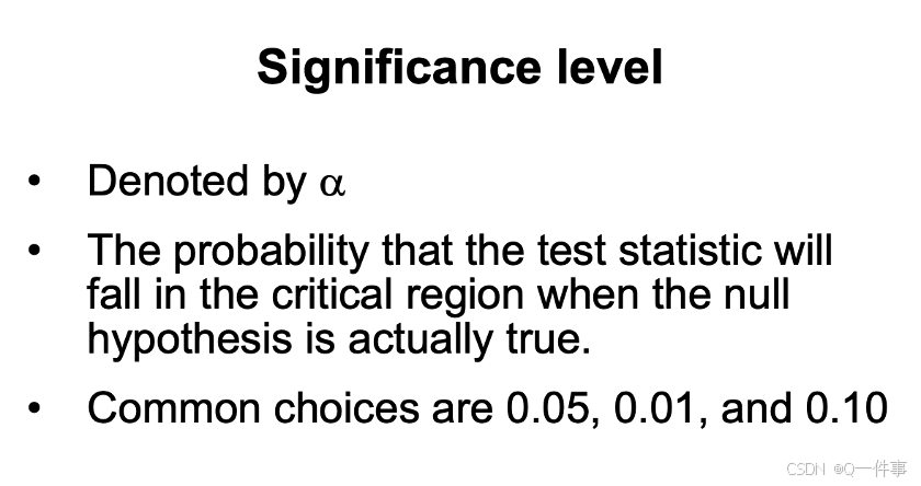
如何陈述

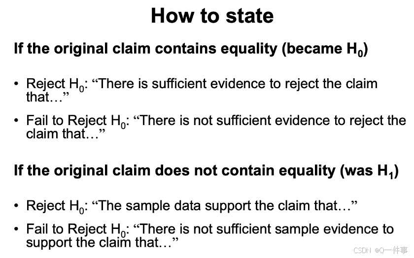
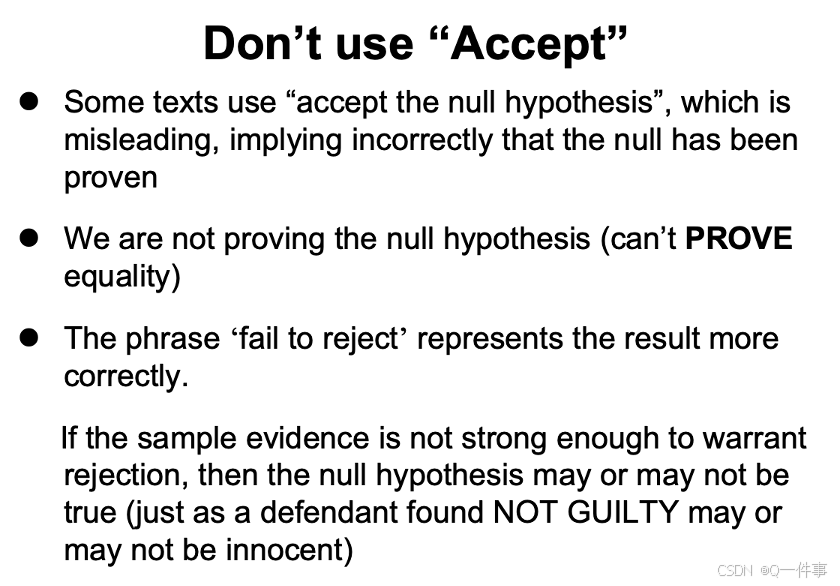
决策和结论

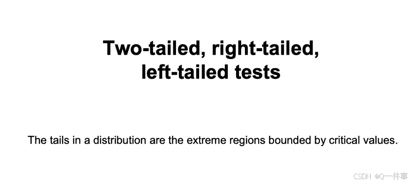
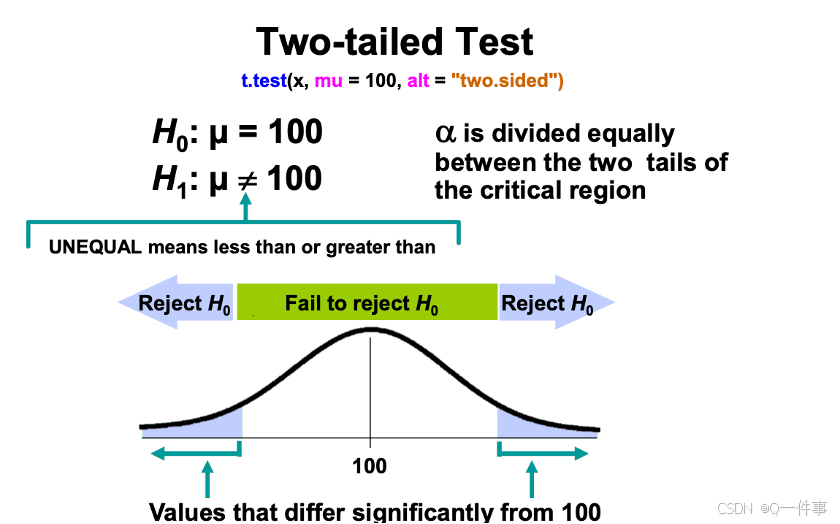
4.假设检验的“双尾”

T检验，分成了两边和左右两个方向

t.test(x, mu = 100, alt = "two.sided")

t.test(x, mu = 100, alt = "two.sided")

t.test(x, mu=100, alt = "greater")

t.test(x, mu=0, alt = "less")

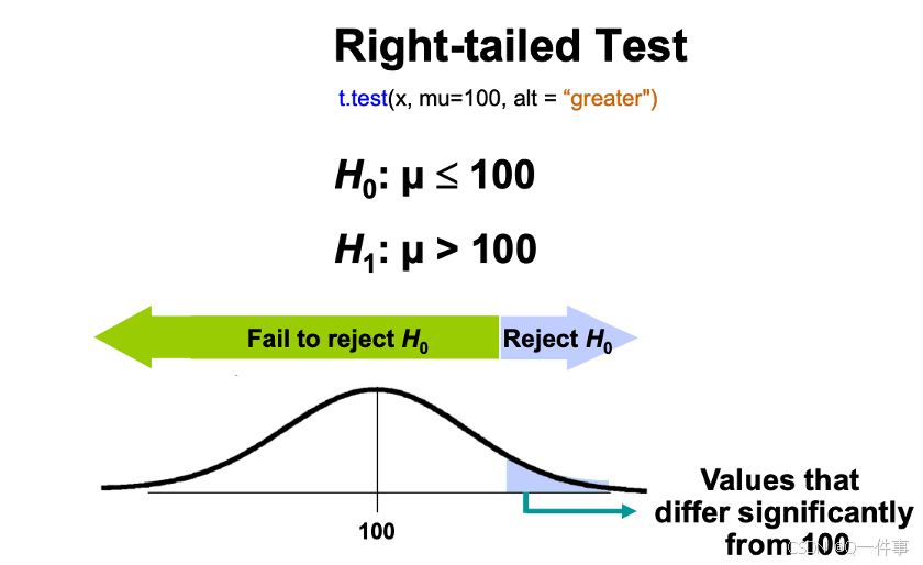
p小于0.05就是可以推翻假设，用单尾可以更好地推翻结论。

前面是概率，后面是自由度。

qt(0.01, 22) # -2.508

prop.test(x, n, p, alternative = c("two.sided", "less", "greater"),conf.level = 0.95, correct = TRUE)
prop.test(0.77*300, 300, p=0.8)

5.配对检验

信息量多用z检验，t检验用于信息量比较。

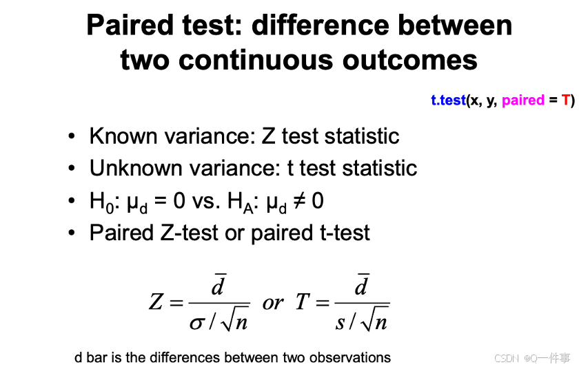
配对检验，更容易有小p值，信息量表征越多，越可能拒绝原假设。

（1）不同情况下计算“双尾”

当方差相等的情况下

t.test(x, y, var.equal = TRUE)

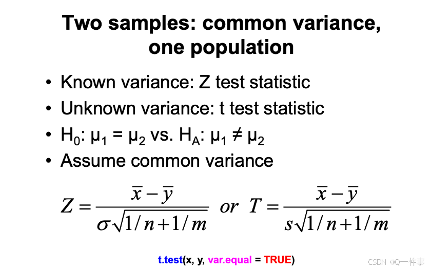
方差不等的情况

t.test(x, y, var.equal = FALSE) # Welch’s t-test

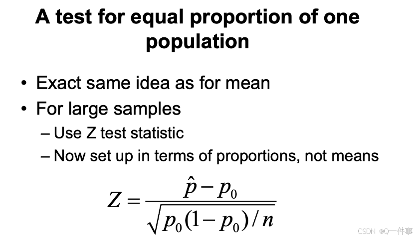
（2）比例关系的检验

比例关系的方差

prop.test(12, 24, p=0.5) # it is a chi square test

两个不同的情况下，比例关系检验

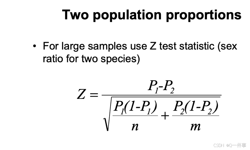
比例关系用的是卡方检验。

x = sample(c('A','B'), 50, rep = T)
y = sample(c('F','M'), 50, rep = T)
table(x,y)

prop.test(table(x,y), correct = TRUE)

# 比例不显著

prop.test(table(x,y), correct = TRUE)
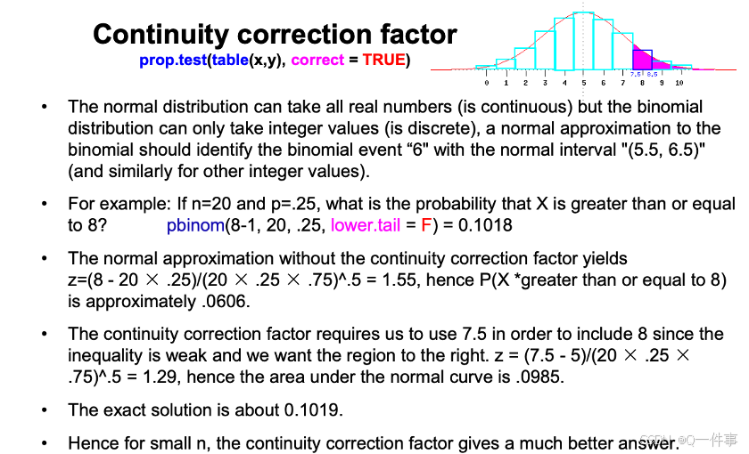
pbinom(8-1, 20, .25, lower.tail = F) = 0.1018

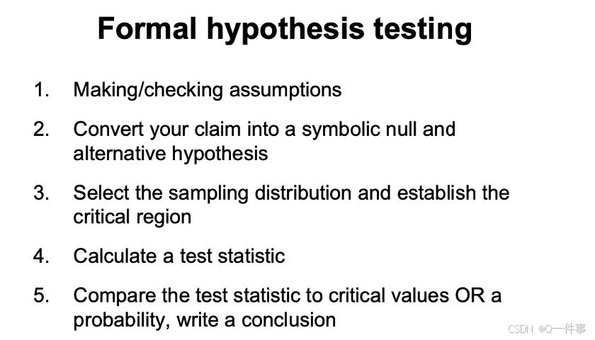
正式假设检验的步骤

最后的公式，（）是单双尾，v是自由度

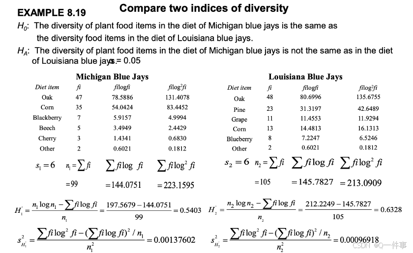
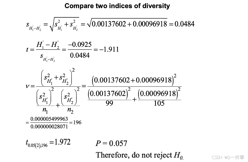
t.test(B, C, var.equal = TRUE)

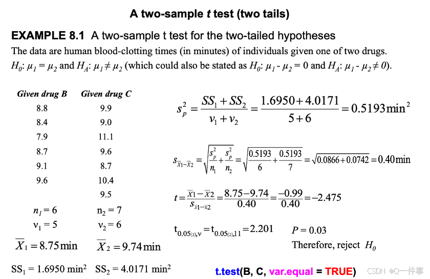
方差的计算，自由度可以

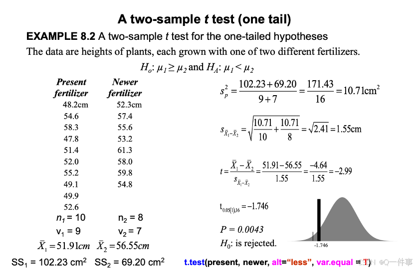
t.test(present, newer, alt=“less”, var.equal = T)

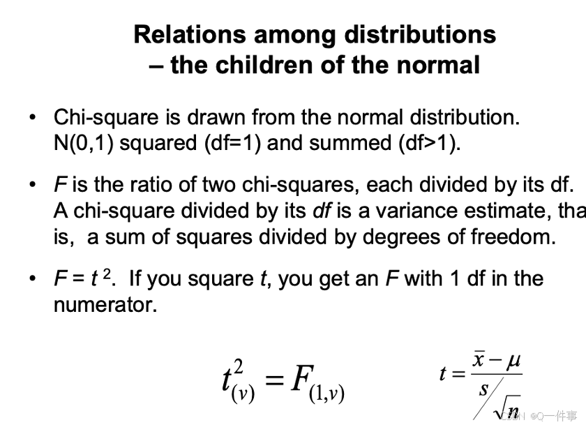
t分布和f分布的关系。

6.作业

7.作业

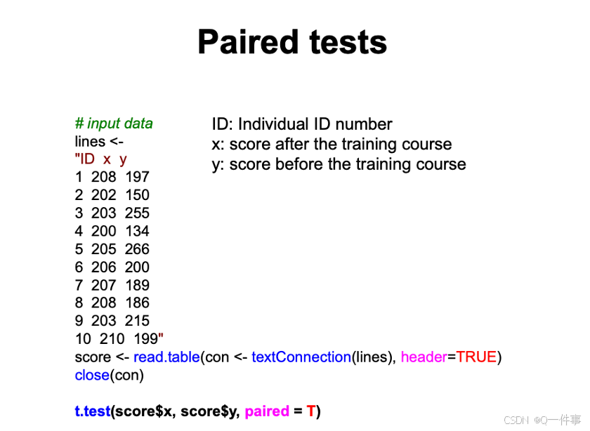
lines <-
"ID x y
1 208 197
2 202 150
3 203 255
4 200 134
5 205 266
6 206 200
7 207 189
8 208 186
9 203 215
10 210 199"
weight <- read.table(con <- textConnection(lines), header=TRUE)
close(con)
# check data
weight
head(weight)

# t test
t.test(weight$x, weight$y, var.equal = F) # two samples
t.test(weight$x, mu = 200) # one sample
shapiro.test(weight$x) # check normal distribution
shapiro.test(weight$y)
hist(weight$y)

因为上面说到了T检验，因而进行回顾一下。

什么是 t 检验？

t 检验也称为 Student t 检验，它是一种使用假设检验来评估一个或两个总体均值的工具。t 检验可用于评估某个组是否与已知值有差异（单样本 t 检验），两个组是否彼此有差异（独立双样本 t 检验），或成对测量值中是否存在显著差异（成对或非独立样本 t 检验）。

如何使用 t 检验？

首先，定义您将要检验的假设，并指定一个可接受的、得出错误结论的风险。例如，比较两个总体时，您可能会假设它们的均值相同，并且您要确定一个可接受的得出错误结论（即不存在差异时认为存在差异）的概率。接下来，您要基于数据计算检验统计量，并将其与来自 t 分布的理论值进行比较。根据结果而定，您要么拒绝原假设，要么无法拒绝原假设。

如果有两个以上的组，该怎么办？

t 检验不适合。请使用多重比较方法。例如：方差分析 (ANOVA)、Tukey-Kramer 配对比较、与单个对照进行比较的 Dunnett’s 检验以及均值分析 (ANOM)。

# Load necessary library
library(ggplot2)

# Define the gravitational constant
G <- 6.67430e-11 # in m^3 kg^-1 s^-2

# Function to calculate gravitational force
gravity_force <- function(m1, m2, r) {
  return(G * (m1 * m2) / r^2)
}

# Define masses and range of distances
m1 <- 5.97e24  # Mass of the Earth in kg
m2 <- 7.35e22  # Mass of the Moon in kg
distance <- seq(1e6, 4e8, by=1e7)  # Distance in meters from 1 million to 400 million meters

# Calculate gravitational forces
force <- gravity_force(m1, m2, distance)

# Create a data frame for plotting
data <- data.frame(distance = distance, force = force)

# Plot the gravitational force vs distance
ggplot(data, aes(x = distance, y = force)) +
  geom_line(color = "blue") +
  labs(title = "Gravitational Force vs Distance",
       x = "Distance (m)",
       y = "Gravitational Force (N)") +
  theme_minimal()