import numpy as np
import pandas as pd
import matplotlib.pyplot as plt
import scipy as sp
from scipy import stats
%matplotlib inline
%config InlineBackend.figure_format = "retina"
from mpl_toolkits.mplot3d import Axes3D
from matplotlib import cm
import matplotlib as mpl
import seaborn as sns
from sklearn.preprocessing import LabelEncoder,OneHotEncoder,normalize,StandardScaler
import warnings
warnings.filterwarnings("ignore")
df=pd.DataFrame(np.random.randn(6,4),columns=list("ABCD"))
df.iloc[2:4,2:4]=np.nan
df.iloc[1,0:2]=np.nan
df
| A | B | C | D |
|---|
| 0 | -0.414608 | 1.303590 | -0.283909 | 2.083562 |
|---|
| 1 | NaN | NaN | 0.922185 | -0.037845 |
|---|
| 2 | 0.854575 | 1.439863 | NaN | NaN |
|---|
| 3 | 0.399861 | -0.650329 | NaN | NaN |
|---|
| 4 | 0.231313 | 1.468190 | 1.626187 | 1.012807 |
|---|
| 5 | 0.776413 | -1.089664 | -0.600983 | -0.667237 |
|---|
df.isnull()
| A | B | C | D |
|---|
| 0 | False | False | False | False |
|---|
| 1 | True | True | False | False |
|---|
| 2 | False | False | True | True |
|---|
| 3 | False | False | True | True |
|---|
| 4 | False | False | False | False |
|---|
| 5 | False | False | False | False |
|---|
df["A"].fillna({'A':0.5},inplace=True)
df["A"]
0   -0.801665
1    0.500000
2    1.582609
3    1.303417
4   -0.442469
5    0.188515
Name: A, dtype: float64
df["B"].fillna(method="bfill")
0    2.154801
1    1.015598
2    1.015598
3    0.470496
4    1.437253
5    0.262288
Name: B, dtype: float64
df["C"].fillna(method="ffill")
0   -0.129508
1    1.358451
2    1.358451
3    1.358451
4   -1.778825
5   -0.354143
Name: C, dtype: float64
df["D"][df["D"].isnull()] = df["D"].mean()
df["D"]
0    0.126941
1    0.012429
2    0.508981
3    0.508981
4    2.337380
5   -0.440826
Name: D, dtype: float64
from sklearn.preprocessing import LabelEncoder,StandardScaler
Iris = pd.read_csv("D:\Desktop\python在机器学习中的应用\Iris.csv")
print(Iris.head(5))
   Id  SepalLengthCm  SepalWidthCm  PetalLengthCm  PetalWidthCm      Species
0   1            5.1           3.5            1.4           0.2  Iris-setosa
1   2            4.9           3.0            1.4           0.2  Iris-setosa
2   3            4.7           3.2            1.3           0.2  Iris-setosa
3   4            4.6           3.1            1.5           0.2  Iris-setosa
4   5            5.0           3.6            1.4           0.2  Iris-setosa
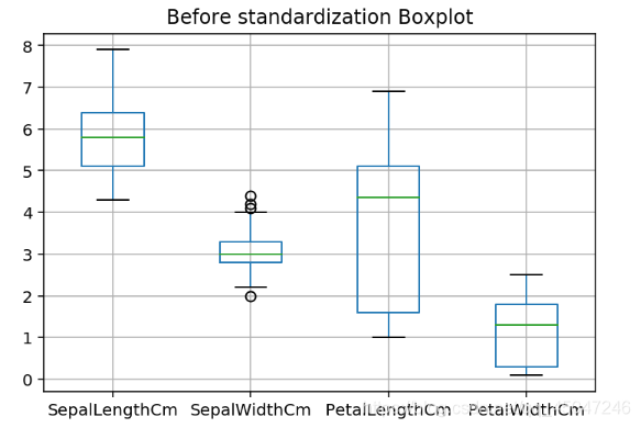
Iris.drop("Id", axis=1).boxplot()
plt.title("Before standardization Boxplot")
plt.show()
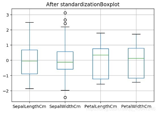
scaler = StandardScaler(with_mean=True,with_std=True)
Iris.iloc[:,1:5] = scaler.fit_transform(Iris.iloc[:,1:5])
Iris.drop("Id", axis=1).boxplot()
plt.title("After standardizationBoxplot")
plt.show()
le = LabelEncoder()
Species = le.fit_transform(Iris.Species)
Species
array([0, 0, 0, 0, 0, 0, 0, 0, 0, 0, 0, 0, 0, 0, 0, 0, 0, 0, 0, 0, 0, 0,
       0, 0, 0, 0, 0, 0, 0, 0, 0, 0, 0, 0, 0, 0, 0, 0, 0, 0, 0, 0, 0, 0,
       0, 0, 0, 0, 0, 0, 1, 1, 1, 1, 1, 1, 1, 1, 1, 1, 1, 1, 1, 1, 1, 1,
       1, 1, 1, 1, 1, 1, 1, 1, 1, 1, 1, 1, 1, 1, 1, 1, 1, 1, 1, 1, 1, 1,
       1, 1, 1, 1, 1, 1, 1, 1, 1, 1, 1, 1, 2, 2, 2, 2, 2, 2, 2, 2, 2, 2,
       2, 2, 2, 2, 2, 2, 2, 2, 2, 2, 2, 2, 2, 2, 2, 2, 2, 2, 2, 2, 2, 2,
       2, 2, 2, 2, 2, 2, 2, 2, 2, 2, 2, 2, 2, 2, 2, 2, 2, 2])
from sklearn.preprocessing import PolynomialFeatures
X = np.arange(8).reshape(4,2)
X
array([[0, 1],
       [2, 3],
       [4, 5],
       [6, 7]])
pf = PolynomialFeatures(degree=2, interaction_only=False, include_bias=False)
pf.fit_transform(X)
array([[ 0.,  1.,  0.,  0.,  1.],
       [ 2.,  3.,  4.,  6.,  9.],
       [ 4.,  5., 16., 20., 25.],
       [ 6.,  7., 36., 42., 49.]])


 被折叠的 条评论
为什么被折叠?
被折叠的 条评论
为什么被折叠?
 到【灌水乐园】发言


