Statistical Thinking in Python (Part 1)笔记

Preface

这是DataCamp的Statistical Thinking in Python (Part 1)笔记，主要内容为利用Python的matplotlib和seaborn等绘图库进行数据可视化

Histogram-Basic

# Import plotting modules
import matplotlib.pyplot as plt
import seaborn as sns

# Set default Seaborn style
sns.set()

# Plot histogram of versicolor petal lengths
_ = plt.hist(versicolor_petal_length)

# Show histogram
plt.show()

Histogram-Adjusting the number of bins

_ = plt.hist(x=versicolor_petal_length, bins=n_bins)

Bea swarm plot

# Create bee swarm plot with Seaborn's default settings
_ = sns.swarmplot(x='species', y='petal length (cm)', data=df)

# Label the axes
_ = plt.xlabel('species')
_ = plt.ylabel('petal length (cm)')

# Show the plot
plt.show()

ECDF（经验累积分布函数）

单变量ECDF

def ecdf(data):
    """Compute ECDF for a one-dimensional array of measurements."""
    # Number of data points: n
    n = len(data)

    # x-data for the ECDF: x
    x = np.sort(data)

    # y-data for the ECDF: y
    y = np.arange(1, n+1) / n
    
    return x,y

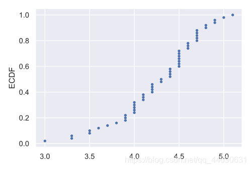
# Compute ECDF for versicolor data: x_vers, y_vers
x_vers, y_vers = ecdf(versicolor_petal_length)

# Generate plot
plt.plot(x_vers,y_vers,marker = '.', linestyle='none')

# Label the axes
plt.xlabel('')
plt.ylabel('ECDF')


# Display the plot
plt.show()

上述代码效果如下：

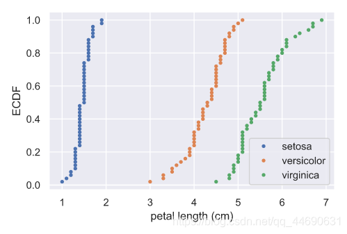
多变量ECDF

# Compute ECDFs
x_set, y_set = ecdf(setosa_petal_length)
x_vers, y_vers = ecdf(versicolor_petal_length)
x_virg, y_virg = ecdf(virginica_petal_length)

# Plot all ECDFs on the same plot
_ = plt.plot(x_set, y_set,marker='.',linestyle='none')
_ = plt.plot(x_vers, y_vers,marker='.',linestyle='none')
_ = plt.plot(x_virg, y_virg,marker='.',linestyle='none')

# Annotate the plot
plt.legend(('setosa', 'versicolor', 'virginica'), loc='lower right')
_ = plt.xlabel('petal length (cm)')
_ = plt.ylabel('ECDF')

# Display the plot
plt.show()

上述代码效果如下：

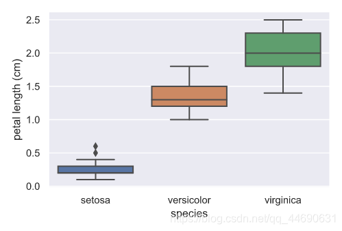
Box-and-whisker plot

# Create box plot with Seaborn's default settings
_ = sns.boxplot(x='species', y='petal length (cm)', data = df)

# Label the axes
_ = plt.xlabel('species')
_ = plt.ylabel('petal length (cm)')

# Show the plot
plt.show()

上述代码效果如下

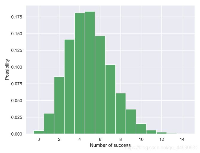
PMF（probability mass function）

在概率论中，概率质量函数 (Probability Mass Function，PMF)是离散随机变量在各特定取值上的概率。

# Compute bin edges: bins
bins = np.arange(0, max(n_defaults) + 1.5) - 0.5

# Generate histogram
_ = plt.hist(n_defaults, bins=bins, normed=True)

# Label axes
_ = plt.xlabel('Number of success')
_ = plt.ylabel('Possibility')

# Show the plot
plt.show()

上述代码效果如下：

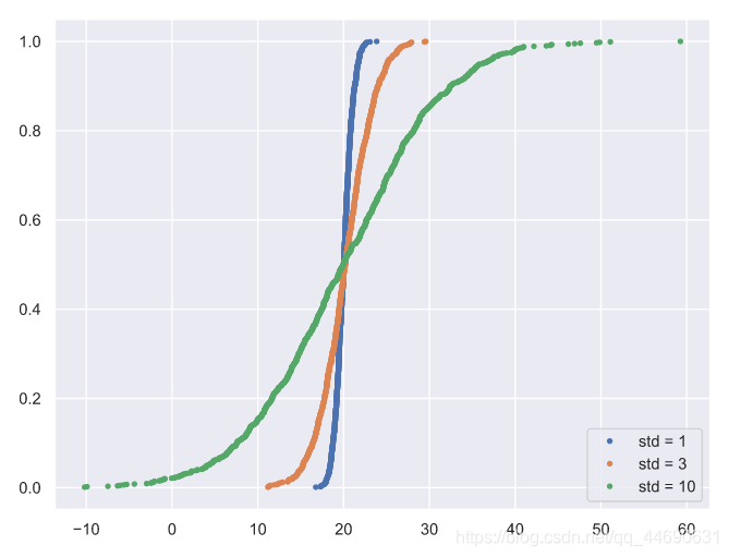
The Normal CDF（正态分布下的累计分布函数）

# Generate CDFs
x_std1, y_std1 = ecdf(samples_std1)
x_std3, y_std3 = ecdf(samples_std3)
x_std10, y_std10 = ecdf(samples_std10)

# Plot CDFs
_ = plt.plot(x_std1, y_std1,marker='.',linestyle='none')
_ = plt.plot(x_std3, y_std3,marker='.',linestyle='none')
_ = plt.plot(x_std10, y_std10,marker='.',linestyle='none')

# Make a legend and show the plot
_ = plt.legend(('std = 1', 'std = 3', 'std = 10'), loc='lower right')
plt.show()

上述代码效果如下：