


活动地址:优快云21天学习挑战赛
1、加载数据
import os,math
from tensorflow.keras.layers import Dropout, Dense, SimpleRNN
from sklearn.preprocessing   import MinMaxScaler
from sklearn                 import metrics
import numpy             as np
import pandas            as pd
import tensorflow        as tf
import matplotlib.pyplot as plt
# 支持中文
plt.rcParams['font.sans-serif'] = ['SimHei']  # 用来正常显示中文标签
plt.rcParams['axes.unicode_minus'] = False  # 用来正常显示负号
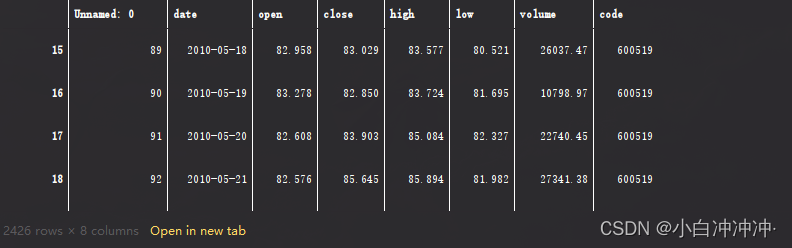
data = pd.read_csv('../data/9/SH600519.csv')  # 读取股票文件
data
"""
前(2426-300=2126)天的开盘价作为训练集,表格从0开始计数,2:3 是提取[2:3)列,前闭后开,故提取出第3列开盘价
后300天的开盘价作为测试集
"""
training_set = data.iloc[0:2426 - 300, 2:3].values
test_set = data.iloc[2426 - 300:, 2:3].values
2、数据预处理
对训练数据进行归一化,加速网络训练收敛。
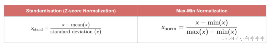
# 训练数据max-min归一化
# from sklearn.preprocessing import MinMaxScaler
sc = MinMaxScaler(feature_range=(0, 1))
training_set = sc.fit_transform(training_set)
test_set = sc.transform(test_set)
设置测试集与训练集
# 设置训练集
x_train = []
y_train = []

x_test = []
y_test = []

"""
使用前60天的开盘价作为输入特征x_train
    第61天的开盘价作为输入标签y_train

for循环共构建2426-300-60=2066组训练数据。
       共构建300-60=260组测试数据
"""
for i in range(60, len(training_set)):
    x_train.append(training_set[i - 60:i, 0])
    y_train.append(training_set[i, 0])

for i in range(60, len(test_set)):
    x_test.append(test_set[i - 60:i, 0])
    y_test.append(test_set[i, 0])

# 对训练集进行打乱
np.random.seed(7)
np.random.shuffle(x_train)
np.random.seed(7)
np.random.shuffle(y_train)
tf.random.set_seed(7)
"""
将训练数据调整为数组(array)

调整后的形状:
x_train:(2066, 60, 1)
y_train:(2066,)
x_test :(240, 60, 1)
y_test :(240,)
"""
x_train, y_train = np.array(x_train), np.array(y_train) # x_train形状为:(2066, 60, 1)
x_test,  y_test  = np.array(x_test),  np.array(y_test)

"""
使x_train和x_test符合RNN输入要求:[送入样本数, 循环核时间展开步数, 每个时间步输入特征个数]。
送入样本数: x_train.shape[0]即2066组数据;
循环核时间展开步数: 输入60个开盘价,
每个时间步输入特征个数:  每个时间步送入的特征是某一天的开盘价,只有1个数据,故为1
"""
x_train = np.reshape(x_train, (x_train.shape[0], 60, 1))
x_test  = np.reshape(x_test,  (x_test.shape[0], 60, 1))
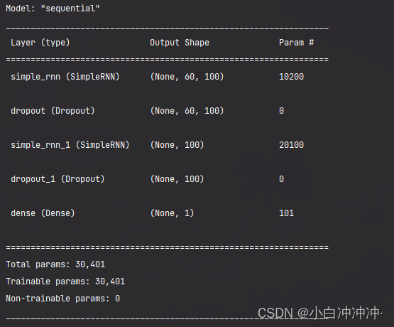
3、构建模型
利用kera创建单隐藏层的RNN模型,并设定模型优化算法adam, 目标函数均方根MSE
# 构建模型
model = tf.keras.Sequential([
    SimpleRNN(100, return_sequences=True), #return_sequences作用是返回输出序列中的最后一个输出(False),还是全部序列(True),默认我False。
    Dropout(0.1),  #防止过拟合
    SimpleRNN(100),
    Dropout(0.1),
    Dense(1)
])
4、激活模型
# 该应用只观测loss数值,不观测准确率,所以删去metrics选项,一会在每个epoch迭代显示时只显示loss值
model.compile(optimizer=tf.keras.optimizers.Adam(0.001),
              loss='mean_squared_error')  # 损失函数用均方误差
5、训练模型
history = model.fit(x_train, y_train,
                    batch_size=64,
                    epochs=20,
                    validation_data=(x_test, y_test),
                    validation_freq=1)                  #测试的epoch间隔数

model.summary()
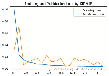
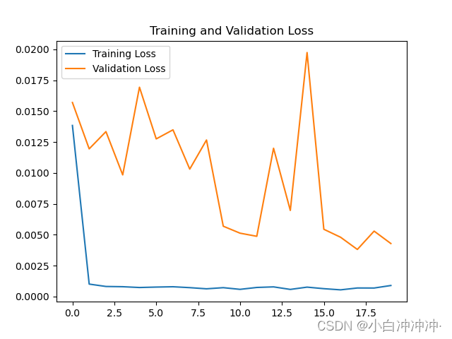
6、结果可视化
plt.plot(history.history['loss']    , label='Training Loss')
plt.plot(history.history['val_loss'], label='Validation Loss')
plt.title('Training and Validation Loss by K同学啊')
plt.legend()
plt.show()
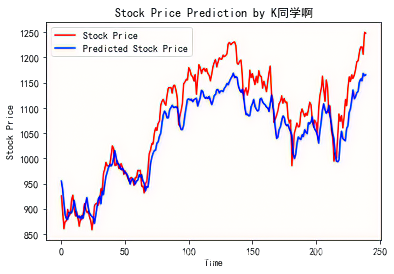
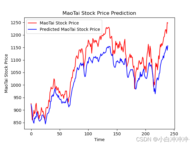
7、预测
predicted_stock_price = model.predict(x_test)                       # 测试集输入模型进行预测
predicted_stock_price = sc.inverse_transform(predicted_stock_price) # 对预测数据还原---从(0,1)反归一化到原始范围
real_stock_price = sc.inverse_transform(test_set[60:])              # 对真实数据还原---从(0,1)反归一化到原始范围

# 画出真实数据和预测数据的对比曲线
plt.plot(real_stock_price, color='red', label='Stock Price')
plt.plot(predicted_stock_price, color='blue', label='Predicted Stock Price')
plt.title('Stock Price Prediction by K同学啊')
plt.xlabel('Time')
plt.ylabel('Stock Price')
plt.legend()
plt.show()
8、评估
"""
MSE  :均方误差    ----->  预测值减真实值求平方后求均值
RMSE :均方根误差  ----->  对均方误差开方
MAE  :平均绝对误差----->  预测值减真实值求绝对值后求均值
R2   :决定系数,可以简单理解为反映模型拟合优度的重要的统计量

详细介绍可以参考文章:https://blog.youkuaiyun.com/qq_38251616/article/details/107997435
"""
MSE   = metrics.mean_squared_error(predicted_stock_price, real_stock_price)
RMSE  = metrics.mean_squared_error(predicted_stock_price, real_stock_price)**0.5
MAE   = metrics.mean_absolute_error(predicted_stock_price, real_stock_price)
R2    = metrics.r2_score(predicted_stock_price, real_stock_price)

print('均方误差: %.5f' % MSE)
print('均方根误差: %.5f' % RMSE)
print('平均绝对误差: %.5f' % MAE)
print('R2: %.5f' % R2)

9、优化
9.1 更改参数
将输入层隐藏单元提升至200个
model = tf.keras.Sequential([
            SimpleRNN(200, return_sequences=True),
            Dropout(0.1),
            SimpleRNN(200),
            Dropout(0.1),
            Dense(1)
结果如下:
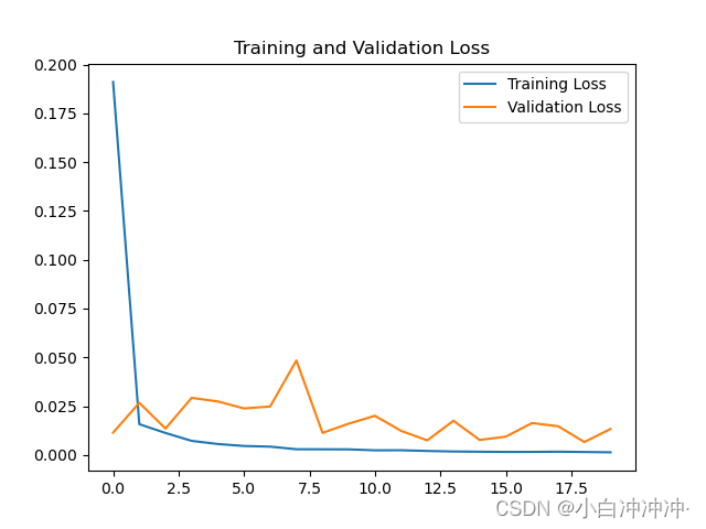

)
均方误差: 6682.101505
均方根误差: 81.744122
平均绝对误差: 75.404096
R2: -0.08172
误差变大,隐藏层为100将Dropout设置为0.2
结果如下:
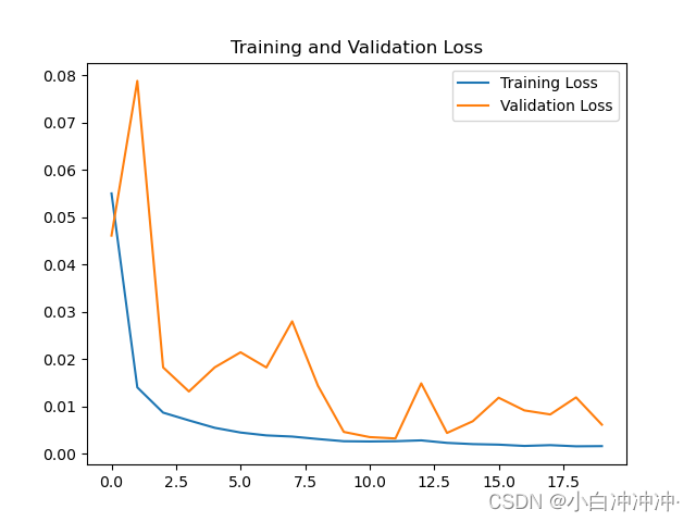
均方误差: 3107.526495
均方根误差: 55.745193
平均绝对误差: 50.249947
R2: 0.57851
参数可以进行慢慢优化(目前有用的是进行更多次的训练),下一步尝试LSTM模型进行优化
9.2利用LSTM模型进行优化尝试
利用LSTM模型进行优化,只需更改model即可
# from tensorflow.keras.layers import Dropout, Dense, SimpleRNN, LSTM
model = tf.keras.Sequential([
            LSTM(100, return_sequences=True),
            Dropout(0.1),
            LSTM(100),
            Dropout(0.1),
            Dense(1)
结果如下
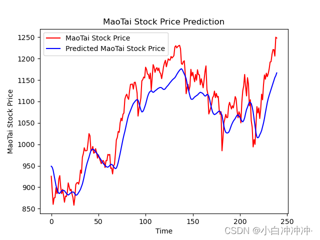
均方误差: 2154.316798
均方根误差: 46.414618
平均绝对误差: 39.309170
R2: 0.71031


 998
998

 被折叠的 条评论
为什么被折叠?
被折叠的 条评论
为什么被折叠?
 到【灌水乐园】发言


