815 LSA LDA文本模型的应用

最新推荐文章于 2024-04-24 15:30:16 发布

端午节放纸鸢

最新推荐文章于 2024-04-24 15:30:16 发布

阅读量864

点赞数 2

文章标签： python

本文链接：https://blog.youkuaiyun.com/qq_43689281/article/details/123882763

版权

815第8周tutorial，主题模型，3个内容

预处理
-数据是sklearn提供的fetch_20newsgroups
-从nltk包下载stopwords，并向stopwords里加入标点符号
-构建一个函数1输入是字符串，功能是去除数字、邮件地址和链接
-对全部的文本数据集实行上述函数
-使用tf-idf vectorizer将原始数据转换成矩阵，要求实行清理函数以及去除数据集最稀有的5%的单词
-输出矩阵的前五个元素以及主要信息
LSA
-LSA的原理
-查看矩阵的维度
-使用sklearn包实施SVD（主成分个数选择20）
-输出对角线元素以及左右正交矩阵
-使用seaborn包绘制对角线元素
-输出每个成分的解释方差以及总的解释方差
-将主成分个数提高
-检查解释方差，绘制图像
-使用散点图对成分进行可视化（optional）
LDA
-去除warning输出（optional） #就是说跑代码的时候会输出很多不重要的warnings，会影响我们看print
-导入LDA包，选择主题数量为10，每个主题的top words的数量是10 # top words大概就是可以代表一个主题的一些单词
-训练LDA模型
-构建一个函数2，输出每个主题的top words
-将主题的数量降低到5，观察区别
-为5个主题取名
-构建一个函数3，输入是训练好的模型、特定的vectoriser、5个主题名称、字符文本，输出是该文本的主题分布
-调用该函数并输出结果
-构建一个函数4，输入是训练好的模型、特定的vectoriser、5个主题名称、top words的数量，输出是每个主题的k top words
-调用该函数并输出结果

实际上这周的tutorial就是使用LSA和LDA进行维度缩减
首先是我们用到的包

# -*- coding: utf-8 -*-
"""
Created on Wed Mar 30 16:51:24 2022

@author: Pamplemousse
"""

import re
import string
import warnings
import numpy as np
import pandas as pd
import seaborn as sns
from matplotlib import pyplot as plt
from nltk.corpus import stopwords
from nltk.tokenize import RegexpTokenizer
from sklearn.datasets import fetch_20newsgroups
from sklearn.decomposition import TruncatedSVD
from sklearn.decomposition import LatentDirichletAllocation as LDA
from sklearn.feature_extraction.text import TfidfVectorizer
#强迫症福音

以及前面提到的四个函数

函数1：
输入为字符串
输出为字符串
功能是去除数字、邮件地址和链接

def rmv_emails_websites(string):
    new_str = re.sub(r"\S+@\S+", '', string) #去除邮件地址
    #以下两个可能是去除链接的，可能它的文本里只有这两种链接（带.co或/和带.ed的）
    new_str = re.sub(r"\S+.co\S+", '', new_str)
    new_str = re.sub(r"\S+.ed\S+", '', new_str)
    new_str = re.sub(r"[0-9]+", '', new_str)
    #去除数字（0到9，但是比如说99，它会当成两个9，然后依次去掉的）
    return new_str

函数2
输入是训练好的模型、特定的vectoriser、top words的数量
没有输出
功能是print每个主题的top words

def print_topics(model, tfidfvectorizer, n_top_words):
    words = tfidfvectorizer.get_feature_names() #得到我们所有的单词（字符型）
    #这个tfidfvectorizer实际上是根据我们的文本数据集构建的转换机制，所以当数据集不一样时，同一篇文章转换出来的矩阵是不一样的。
    for topic_idx, topic in enumerate(model.components_):
    #topic_idx是topic的索引
        print("\nTopic #%d: " % topic_idx)
        print(" ".join([words[i] for i in topic.argsort()[:-n_top_words - 1:-1]]))
        #注意，双引号中间有空格，这样输出后才好看，否则单词会粘在一起
        #第二个print值得一讲
'''
首先这里有个topic.argsort(),这个函数呢，它就把topic里面的单词从小到大排序（由于这里
经过了tfidf转换，所以是代表单词在主题下的重要程度的数值型数据,所以可以排序）排序好以后，每个位置存的是当前的位次原先所在的索引，然后[:-n_top_words - 1:-1]就代表经过排序
后的topic里的倒数第n_top_words（-(n_top_words+1)）开始的单词直到最后一个单词，也就
是说这里输出的是前n_top_words个单词。
然后，topic.argsort()[:-n_top_words - 1:-1]，输出的就是n个top words原本的索引（int型）
最后在words里面找到这个单词（string）
'''

函数3
输入是训练好的模型、vectorizer、主题的名称、文本字符串
输出是该文本每个主题的分布情况

def get_inference(model, vectorizer, topics, text):
    v_text = vectorizer.transform([text])
    #首先把字符文本使用我们已经构建好的转换规则进行转换->矩阵
    score = model.transform(v_text)
    #然后将矩阵放入模型得到该文本每个主题的分布
    return topics[np.argmax(score)], score

函数4
输入是训练好的模型、vectorizer、主题的名称、top words的数量
输出是每个主题的top words

#注意这里给top words的数量赋值为15了，就是说我们在调用这个函数的时候如果没有给第四个输入那么就默认是15，如果给了，给的是多少就是多少
def get_model_topics(model, vectorizer, topics, n_top_words=15):
    word_dict = {} #声明一个单词字典
    feature_names = vectorizer.get_feature_names()
    for topic_idx, topic in enumerate(model.components_):
        top_features_ind = topic.argsort()[:-n_top_words - 1: -1]
        #这里又是得到某个主题的top words的索引（这里是数值型）
        top_features = [feature_names[i] for i in top_features_ind]
        #top words对应的单词
        word_dict[topics[topic_idx]] = top_features
        #将第i个主题的top words写入字典
    return pd.DataFrame(word_dict)

Task 1: 数据预处理

#导入fetch_20newsgroups训练数据
X_train, y_train = fetch_20newsgroups(subset='train', return_X_y=True)
#输出第一个数据
print(X_train[0]) #输出1

#构建stopwords
tokenizer = RegexpTokenizer(r'\b\w{3,}\b')
stop_words = list(set(stopwords.words("english")))#从nltk下载stopwords
stop_words += list(string.punctuation)#通过添加标点符号扩建stopwords

#输出stopwords
print(stop_words) #输出2

#调用函数1
X_train = list(map(rmv_emails_websites, X_train))

#使用tfidf将原始数据转换成矩阵
tfidf = TfidfVectorizer(lowercase=True,
                        stop_words=stop_words,
                        tokenizer=tokenizer.tokenize,
                        min_df=0.05#去掉频率最低的5%的数据
                        )#构建tfidfvectorizer参数
tfidf_train_sparse = tfidf.fit_transform(X_train)#使用tfidf拟合并转换数据
tfidf_train_df = pd.DataFrame(tfidf_train_sparse.toarray(),
                              columns=tfidf.get_feature_names())#用单词（string）标记列名
                              #将转换后的数据换成dataframe形式
print(tfidf_train_df.head())#输出3前五个元素

print(tfidf_train_df.info())#输出4矩阵的主要信息

输出1:

From: lerxst@wam.umd.edu (where’s my thing) Subject: WHAT car is
this!? Nntp-Posting-Host: rac3.wam.umd.edu Organization: University of
Maryland, College Park Lines: 15

I was wondering if anyone out there could enlighten me on this car I
saw the other day. It was a 2-door sports car, looked to be from the
late 60s/ early 70s. It was called a Bricklin. The doors were really
small. In addition, the front bumper was separate from the rest of the
body. This is all I know. If anyone can tellme a model name, engine
specs, years of production, where this car is made, history, or
whatever info you have on this funky looking car, please e-mail.

Thanks,

IL ---- brought to you by your neighborhood Lerxst ----

因为这里还没有调用函数1，所以我们还能看到邮件地址和数字

输出2：

[‘this’, “didn’t”, ‘about’, ‘them’, ‘mustn’, ‘him’, ‘when’, ‘will’, ‘between’, ‘t’, “should’ve”, ‘itself’, ‘over’, ‘under’, ‘for’, ‘so’, ‘than’, “she’s”, ‘being’, ‘hasn’, “that’ll”, ‘ourselves’, ‘my’, ‘aren’, ‘in’, ‘ma’, ‘to’, ‘did’, ‘they’, ‘his’, ‘do’, “you’d”, ‘only’, ‘why’, ‘by’, ‘all’, ‘an’, ‘after’, ‘where’, ‘doing’, “it’s”, ‘o’, ‘few’, ‘shan’, ‘yourselves’, ‘was’, ‘mightn’, ‘weren’, ‘what’, “aren’t”, ‘ll’, ‘been’, ‘don’, ‘above’, ‘too’, ‘am’, ‘she’, ‘had’, ‘s’, ‘ain’, ‘hadn’, ‘no’, ‘isn’, ‘needn’, ‘won’, ‘me’, ‘but’, ‘while’, ‘both’, ‘haven’, ‘should’, ‘until’, “couldn’t”, ‘during’, ‘having’, ‘themselves’, ‘each’, “won’t”, ‘just’, ‘have’, ‘nor’, ‘any’, “doesn’t”, “shan’t”, ‘their’, “shouldn’t”, ‘how’, ‘such’, ‘its’, ‘out’, ‘doesn’, ‘those’, ‘himself’, ‘and’, ‘y’, ‘again’, ‘against’, ‘who’, ‘we’, ‘these’, “wouldn’t”, ‘i’, ‘didn’, ‘wouldn’, “don’t”, ‘before’, ‘because’, ‘yours’, ‘very’, ‘herself’, ‘whom’, ‘is’, ‘the’, ‘same’, “weren’t”, ‘below’, ‘be’, ‘d’, ‘most’, ‘which’, ‘it’, ‘own’, ‘shouldn’, ‘more’, ‘off’, ‘her’, ‘here’, ‘on’, ‘some’, ‘further’, ‘he’, ‘or’, ‘yourself’, ‘couldn’, ‘up’, ‘our’, ‘there’, ‘re’, ‘wasn’, ‘can’, ‘that’, “you’re”, “you’ll”, ‘does’, ‘theirs’, ‘a’, ‘myself’, ‘other’, ‘through’, ‘once’, “mustn’t”, ‘down’, ‘not’, “hasn’t”, ‘of’, ‘from’, “you’ve”, ‘with’, ‘if’, ‘your’, ‘ve’, ‘m’, ‘as’, “needn’t”, ‘are’, ‘has’, ‘you’, “hadn’t”, “isn’t”, ‘hers’, ‘were’, ‘into’, “haven’t”, ‘now’, ‘ours’, ‘at’, “mightn’t”, “wasn’t”, ‘then’, ‘!’, ‘"’, ‘#’, ‘$’, ‘%’, ‘&’, “’”, ‘(’, ‘)’, ‘*’, ‘+’, ‘,’, ‘-’, ‘.’, ‘/’, ‘:’, ‘;’, ‘<’, ‘=’, ‘>’, ‘?’, ‘@’, ‘[’, ‘\’, ‘]’, ‘^’, ‘_’, ‘`’, ‘{’, ‘|’, ‘}’, ‘~’]

没什么好说的

输出3：

able access actually ago … year years yes yet
0 0.0 0.000000 0.000000 0.0 … 0.0 0.129397 0.000000 0.000000
1 0.0 0.000000 0.000000 0.0 … 0.0 0.000000 0.000000 0.000000
2 0.0 0.131975 0.121422 0.0 … 0.0 0.000000 0.000000 0.000000
3 0.0 0.000000 0.000000 0.0 … 0.0 0.000000 0.000000 0.000000
4 0.0 0.000000 0.000000 0.0 … 0.0 0.000000 0.237686 0.237104
[5 rows x 241 columns]

第一行是列名，表示每一列所对应的单词，第一列是文章索引，中间的数据是矩阵，可以看到前五个文本都没有able这个单词（amazing），第一篇文章有years，第三篇文章有access和actually，第五篇文章有yes和yet
然后我们还可以看出，我们的模型有241个单词

输出4：

<class ‘pandas.core.frame.DataFrame’>
RangeIndex: 11314 entries, 0 to 11313
Columns: 241 entries, able to yet
dtypes: float64(241)
memory usage: 20.8 MB
None

这个输出是我们矩阵的主要信息
首先我们矩阵的数据类型是dataframe
然后我们有11314行，241列，所以我们有11314个文本和用了241个单词来表示
存储的数据类型是双精度浮点数（就跟C++里的double是一个意思）
数据存储大小是20.8MB

任务2：LSA
首先老师给了很多图来讲SVD和LSA，这里我们就不讲了，网上很多嘛，这里偷一个SVD链接
我们直接看LSA实践

#看看我们有多少列，避免我们选择的主成分个数多于全部成分的个数
print('Number of columns in our dataset is:', len(tfidf_train_df.columns))
#输出1
print(tfidf_train_df.head(10))
#输出2

#选择主成分的个数为20
svd = TruncatedSVD(n_components=20, n_iter=100, random_state=42)

#进行奇异值分解
sample_decomp = svd.fit_transform(tfidf_train_df.to_numpy())
Sigma = svd.singular_values_
U = sample_decomp/Sigma
V_T = svd.components_

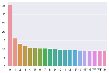
#使用seaborn绘制对角线元素
#barplot即为柱状图，横轴是第i个对角线元素，纵轴是第i个对角线元素的值
sns.barplot(x=list(range(len(Sigma))), y = Sigma)#图0

#左正交矩阵的维度
print(U.shape)#输出3
#右正交矩阵的维度
print(V_T.shape)#输出4

#每个成分的解释方差
print(svd.explained_variance_ratio_)#输出5
#总的解释方差
print(svd.explained_variance_ratio_.sum())#输出6

#将主成分个数提高到100
skl_decomp_obj = TruncatedSVD(n_components=100, n_iter=100, random_state=42)
tfidf_lsa_data = skl_decomp_obj.fit_transform(tfidf_train_df)

print(tfidf_lsa_data.shape)#输出7
#输出总的解释方差
print(skl_decomp_obj.explained_variance_ratio_.sum())#输出8

#绘制解释方差和主成分个数的关系图
plt.figure()
plt.plot(np.cumsum(skl_decomp_obj.explained_variance_ratio_))
plt.xlabel('Number of Components')
plt.ylabel('Variance (%)')
plt.title('Newgroups TF-IDF Dataset Explained Variance')
plt.show()#图1

#利用散点图对成分进行可视化
sns.scatterplot(tfidf_lsa_data[:,0], tfidf_lsa_data[:,1])
plt.show();#图2
sns.scatterplot(tfidf_lsa_data[:,0], tfidf_lsa_data[:,2])
plt.show();#图3
sns.scatterplot(tfidf_lsa_data[:,1], tfidf_lsa_data[:,2])
plt.show();#图4

fig = plt.figure(figsize=(10,10))
ax = fig.add_subplot(111, projection='3d')
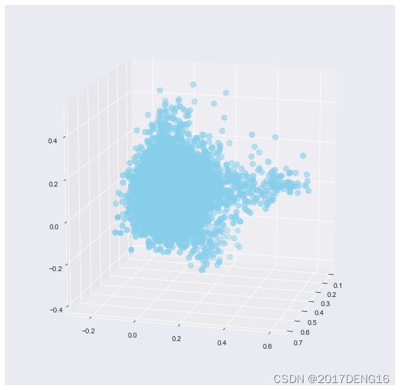
ax.scatter(tfidf_lsa_data[:,0], tfidf_lsa_data[:,15], tfidf_lsa_data[:,9], c='skyblue', s=60)
ax.view_init(15,15)
plt.show()#图5

输出1：

Number of columns in our dataset is: 241

输出2：

able access actually ago … year years yes yet
0 0.0 0.000000 0.000000 0.0 … 0.000000 0.129397 0.000000 0.000000
1 0.0 0.000000 0.000000 0.0 … 0.000000 0.000000 0.000000 0.000000
2 0.0 0.131975 0.121422 0.0 … 0.000000 0.000000 0.000000 0.000000
3 0.0 0.000000 0.000000 0.0 … 0.000000 0.000000 0.000000 0.000000
4 0.0 0.000000 0.000000 0.0 … 0.000000 0.000000 0.237686 0.237104
5 0.0 0.118014 0.000000 0.0 … 0.104030 0.000000 0.000000 0.000000
6 0.0 0.000000 0.000000 0.0 … 0.000000 0.000000 0.000000 0.000000
7 0.0 0.000000 0.000000 0.0 … 0.000000 0.000000 0.000000 0.000000
8 0.0 0.000000 0.000000 0.0 … 0.000000 0.000000 0.000000 0.000000
9 0.0 0.000000 0.000000 0.0 … 0.172097 0.000000 0.000000 0.000000

图0：
对角线元素
输出3：

(11314, 20)

输出4：

(20, 241)

就是说原本的矩阵(11314, 241)被分解成了(11314, 20) (20, 20) (20, 241)

输出5：

[0.00631212 0.0258966 0.01679788 0.01374899 0.01190696 0.01118847
0.01074829 0.01052689 0.0103112 0.00963623 0.00937076 0.00910335
0.00883867 0.00852629 0.00843441 0.00840878 0.00810704 0.00802402
0.00795814 0.00778352]

输出6：

0.21162860943916073

输出7：

(11314, 100)

输出8：

0.6217337133713389

图1：主成分个数和解释方差的关系
主成分个数与解释方差的关系

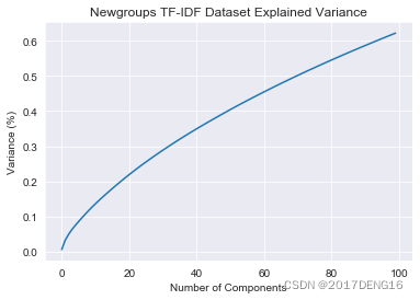
图2：1号主成分和2号主成分之间的散点图
横轴为1号主成分，纵轴为2号主成分

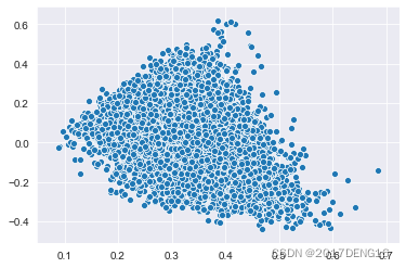
图3：1号主成分和3号主成分之间的散点图
在这里插入图片描述
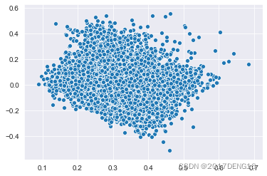
图4：2号主成分和3号主成分之间的散点图

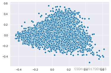
图5：1号16号10号主成分之间的3d图
在这里插入图片描述

说完我们还是没懂LSA是什么，不过没关系，我们下面看LDA（狗头）

#将主题个数设为10，top words数量设为10
number_topics = 10
number_words = 10
#使用上述参数训练lda
lda = LDA(n_components=number_topics, n_jobs=-1, random_state=1)
lda.fit(tfidf_train_df)
#输出1
print("Topics found via LDA:")
print_topics(lda, tfidf, number_words)

#将主题个数降到5
number_topics = 5
number_words = 10
lda = LDA(n_components=number_topics, n_jobs=-1, random_state=1)
lda.fit(tfidf_train_df)
#输出2
print("Topics found via LDA:")
print_topics(lda, tfidf, number_words)

#取5个主题名字
lda_topics = ['space.data', 'religion.artc', 'uni.org', 'law.gow', 'car.org']

#一个随机的文本example
text = 'Google said on Thursday that it signed a deal with Elon Musk’s SpaceX to use the space company’s growing satellite internet service, Starlink, with its cloud unit. SpaceX will install Starlink terminals at Google’s cloud data centers around the world, aiming to utilize the cloud for Starlink customers and enabling Google to use the satellite network’s speedy internet for its enterprise cloud customers'
#调用get_inference函数获取文本主题分布
topic, score = get_inference(lda, tfidf, lda_topics, text)
print(topic, score)#输出3

#调用get_model_topics
print(get_model_topics(lda, tfidf, lda_topics))#输出4

输出1

Topics found via LDA:

Topic #0: data version bit newsreader use number subject one lines
system

Topic #1: institute technology research center posting nntp host
subject lines organization

Topic #2: windows program problem using use lines help subject access
organization

Topic #3: government law people public would writes article state
organization subject

Topic #4: car computer science article writes organization subject
lines university one

Topic #5: year article writes one last would years time subject like

Topic #6: thanks university subject lines organization posting please
host nntp mail

Topic #7: space david list organization subject lines apr article
posting writes

Topic #8: god people one would writes article think believe say know

Topic #9: drive power article lines writes organization subject left
host posting

输出2：

Topics found via LDA:

Topic #0: drive space research data lines subject center organization
david posting

Topic #1: god year one writes article last would subject lines
organization

Topic #2: windows subject lines organization university thanks
posting host nntp please

Topic #3: people would writes one article government think law like
subject

Topic #4: writes article car one would organization subject lines
like get

输出3：

space.data [[0.76349816 0.05887915 0.05980328 0.05874562 0.05907379]]

就是说这篇文本被认为是第一类里面的

输出4：
space.data religion.artc uni.org law.gow car.org
0 drive god windows people writes
1 space year subject would article
2 research one lines writes car
3 data writes organization one one
4 lines article university article would
5 subject last thanks government organization
6 center would posting think subject
7 organization subject host law lines
8 david lines nntp like like
9 posting organization please subject get
10 university think mail lines university
11 host people card organization good
12 nntp time distribution right posting
13 article good anyone know host
14 number years know get nntp

5个主题的默认15个stopwords
这个输出在控制台上看起来还是很好看的，就是说这里懒得截图了。

别催了别催了
下班