


全连接神经网络是深度学习入门必学的网络,今天我们来看一个两层的全连接神经网络的搭建过程,以及实现图片的预测,先看一张图: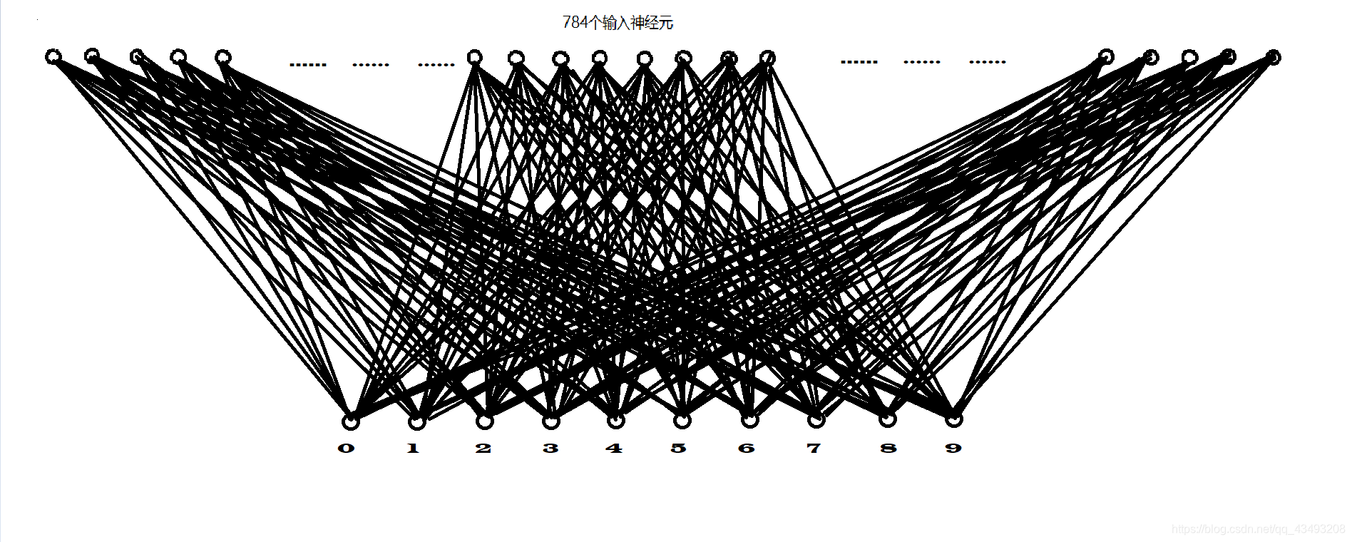
这张图是一个输入层为784个神经元,输出层为10个神经元的两层的全连接,(我的好兄弟说它像蝙蝠,确实有点像,更像的或许是谈到神经网络和谈到蝙蝠时我们内心的凝重,希望疫情早日结束),这个图是我画来表示一个使用mnist数据集训练手写数字识别的神经网络,而我们在程序里用到的是输入层有4900个神经元,输出层7个类别的神经网络,所有的训练样本都会被展开为一个1*4900的向量输入到网络中。在上面一篇博客中我们已经说过深度学习的四个步骤1.数据准备 2.搭建模型 3.训练模型 4.保存和使用模型 下面看代码
# * coding:utf-8 *
# 作者:Little Bear
# 创建时间:2020/2/4 9:19
import tensorflow as tf
import pylab
from skimage import io, transform
import os
import numpy as np
import glob

# 第一步:数据准备阶段 对虚汗连样本中的数据进行大小归一化,构建训练样本tensor
# 设置训练样本图片的路径train_path 设置模型的存储路径model_path
tf.reset_default_graph()
train_path = 'data/hand-images/'
model_path = 'model/classification.ckpt'
# 设置图片归一化的尺度70*70
w = 70
h = 70


# 读取图片,图片的归一化处理
def read_img(path):
    image_folder = [train_path + folder for folder in os.listdir(train_path) if os.path.isdir(train_path + folder)]
    images = []
    labels = []
    for index, folder in enumerate(image_folder):
        print("正在读取第 %d 个文件夹" % index, " 文件夹的名字是:%s" % folder)
        for im in glob.glob(folder + '/*.jpg'):
            print('reading the image : %s' % im)
            # 读取图片
            img = io.imread(im, as_gray=True)
            # 调整图片的大小
            img = transform.resize(img, (w, h))
            # 将图片加入图片集合
            images.append(img)
            # 将图片对应的标签加入样本集合
            labels.append(index)
    return np.asarray(images, np.float32), np.asarray(labels, np.int32)


def doLabelArray(labels, number):
    array = np.zeros((number, 7), np.int32)
    for i in range(number):
        array[i][labels[i]] = 1
    return array


# 读取图片,归一化处理
data, label = read_img(train_path)
# 图片的数量
train_number = data.shape[0]
# 对图片的顺序进行打乱
arr = np.arange(train_number)
np.random.shuffle(arr)
data = data[arr]
label = label[arr]
# 设置训练数据和测试数据的数量
label = doLabelArray(label, 1599)
print(label)
ratio = 0.9
s = np.int(train_number * ratio)
x_train = data[:s]
y_train = label[:s]
x_test = data[s:]
y_test = label[s:]
# 第二步:搭建模型
x = tf.placeholder(tf.float32, [None, 4900])
y = tf.placeholder(tf.float32, [None, 7])
W = tf.Variable(tf.random_normal([4900, 7]))
b = tf.Variable(tf.zeros([7]))
pred = tf.nn.softmax(tf.matmul(x, W) + b)
print(pred)
cost = tf.reduce_mean(-tf.reduce_sum(y * tf.log(pred+pow(10.0, -9)), reduction_indices=1))
#此处有一个很重要的问题,就是损失出现了nan,这里加了一个极小值
learn_rate = 0.05
optimizer = tf.train.GradientDescentOptimizer(learn_rate).minimize(cost)
train_epochs = 50
batch_size = 80
saver = tf.train.Saver()
# 第三步:开始训练
with tf.Session() as sess:
    sess.run(tf.global_variables_initializer())
    for i in range(train_epochs):
        avg_cost = 0.1
        total_batch = int(train_number * 0.9 / batch_size)
        for j in range(total_batch):
            batch_x = x_train[(j) * batch_size:(j + 1) * batch_size]
            batch_y = y_train[(j) * batch_size:(j + 1) * batch_size]
            _, c = sess.run([optimizer, cost], feed_dict={x: np.reshape(batch_x, [80, 4900]), y: batch_y})
            avg_cost += c / total_batch
        if (i + 1) % 1 == 0:
            print("Epoch:", '%04d' % (i + 1), "cost=", "{:.9f}".format(avg_cost))
    print("finished!")
    correct_prediction = tf.equal(tf.argmax(pred, 1), tf.argmax(y, 1))
    accuracy = tf.reduce_mean(tf.cast(correct_prediction, tf.float32))
    print("Accuracy:", accuracy.eval({x: np.reshape(x_test, [160, 4900]), y: y_test}))

    # Save model weights to disk
    save_path = saver.save(sess, model_path)
    print("Model saved in file: %s" % save_path)
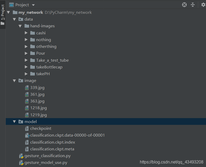
项目目录结构
第一步:数据准备阶段
在数据准备阶段我们将所有的训练图片进行归一化,所有的图片必须具有相同的大小,我这全部设置为了7070,训练图片的像素越大网络的参数也就会越多,训练的时间也就会慢一些(不过我们暂时不用考虑这个问题,毕竟我们就两层。。。),我这里将所有的图片都转化为了灰度图,将所有的图片都转化为数组后加入到images列表然后转化为ndarray数据类型返回到data中,此时data的形状应该是n7070,以图片在不同的文件夹来区分不同的类别,labels后续还要做进一步的处理,转化为n7的数组,(n代表图片的数量)。这样数据准备阶段基本完成。
第二步:模型的搭建过程
1…首先我们应该考虑的是模型的入口,
x = tf.placeholder(tf.float32, [None, 4900])
y = tf.placeholder(tf.float32, [None, 7])
这两句代码设置了训练过程中模型的入口,x代表输入的图片的矩阵,y代表输入图片对应的标签,使用的是tensorflow中的占位符的方法,tf.float32代表需要的数组的数据类型,中括号[ ]中的数代表数组的规模,其中None代表可以为任意大小的数。
2.然后设置好模型的参数
W = tf.Variable(tf.random_normal([4900, 7]))
b = tf.Variable(tf.zeros([7]))
W为全连接网络的权重,b为偏置值。
4.最后设置好激活函数,和梯度下降操作。
pred = tf.nn.softmax(tf.matmul(x, W) + b)
print(pred)
cost = tf.reduce_mean(-tf.reduce_sum(y * tf.log(pred+pow(10.0, -9)), reduction_indices=1))
learn_rate = 0.05
optimizer = tf.train.GradientDescentOptimizer(learn_rate).minimize(cost)
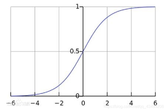
值得注意的是这里使用softmax作为激活函数,softmax会把输入的值映射到(0,1),并且所有的输出神经元的值相加和为1,很好的用于分类任务。下图为softmax图像:
第三步:训练模型
训练模型的过程要注意,训练样本是分批进行训练的,这补充一下,训练样本要打乱顺序,【因为随机梯度下降一批一批的输入数据,如果一批的数据都很类似的话容易导致换批的时候梯度变化太大】,这句话是我的老师说的,我也不太懂。。。总之打乱再训练就对了。
第四步:保存和使用模型
下面的代码是模型的使用:
# * coding:utf-8 *
# 作者:Little Bear
# 创建时间:2020/2/5 8:59
# 读取模型
import pylab
import tensorflow as tf
import glob
import numpy as np
from skimage import io, transform


def readImage(image_path):
    images = []
    for path in glob.glob(image_path):
        print(path)
        image = io.imread(path,as_gray=True)
        image = transform.resize(image, (70, 70))
        images.append(image)
    return np.asarray(images, np.float32)


model_path = 'model/classification.ckpt'
image_path = 'image/*.jpg'
test = readImage(image_path)
print(test)
x = tf.placeholder(tf.float32, [None, 4900])
y = tf.placeholder(tf.float32, [None, 7])
W = tf.Variable(tf.random_normal([4900, 7]))
b = tf.Variable(tf.zeros([7]))
pred = tf.nn.softmax(tf.matmul(x, W) + b)
cost = tf.reduce_mean(-tf.reduce_sum(y * tf.log(pred + pow(10.0, -9)), reduction_indices=1))
learn_rate = 0.05
optimizer = tf.train.GradientDescentOptimizer(learn_rate).minimize(cost)
train_epochs = 50
batch_size = 80
saver = tf.train.Saver()
print("Starting 2nd session...")
with tf.Session() as sess:
    # Initialize variables
    sess.run(tf.global_variables_initializer())
    # Restore model weights from previously saved model
    saver.restore(sess, model_path)

    # 测试 model
    correct_prediction = tf.equal(tf.argmax(pred, 1), tf.argmax(y, 1))
    # 计算准确率
    # accuracy = tf.reduce_mean(tf.cast(correct_prediction, tf.float32))
    # print("Accuracy:", accuracy.eval({x: mnist.test.images, y: mnist.test.labels}))

    output = tf.argmax(pred, 1)
    # batch_xs, batch_ys = mnist.train.next_batch(2)
    outputval, predv = sess.run([output, pred], feed_dict={x:np.reshape(test,[5,4900])})
    print(outputval)

    im = test[0]
    im = im.reshape(-1, 28)
    pylab.imshow(im)
    pylab.show()

    im = test[1]
    im = im.reshape(-1, 28)
    pylab.imshow(im)
    pylab.show()
两层的全连接网络能力并不强,如果想要更准确的分类应该采用更复杂的网络。如需整个项目资源包括训练样本可自行下载,如果没有积分可以私信联系我邮箱发给你。如有错误请多指正。


 1562
1562

 被折叠的 条评论
为什么被折叠?
被折叠的 条评论
为什么被折叠?
 到【灌水乐园】发言


