


1. 加载数据集和所需的包,检查输入数据
library(Seurat)
library(tidyverse)
library(cowplot)
library(patchwork)
library(WGCNA)
library(hdWGCNA)
theme_set(theme_cowplot())
set.seed(12345)
enableWGCNAThreads(nThreads = 8)

seurat_obj <- readRDS('yourdata.rds')
p <- DimPlot(seurat_obj, group.by='cell_type', label=TRUE) +
   umap_theme() + ggtitle('Zhou et al Control Cortex') + NoLegend()
p
2. 设置seurat对象
gene_select方式有三种:
variable:使用存储在 Seurat 对象的 VariableFeatures 中的基因;
fraction:使用在整个数据集或每组细胞中以一定比例的细胞表达的基因,由 group.by 指定;
custom:使用自定义列表中指定的基因。
seurat_obj <- SetupForWGCNA(
  seurat_obj,
  gene_select = "fraction",
  fraction = 0.05,
  wgcna_name = "tutorial"
)
3. 构建metacell
seurat_obj <- MetacellsByGroups(
  seurat_obj = seurat_obj,
  group.by = c("cell_type", "Sample"),
  reduction = 'harmony', # 'umap','tsne'
  k = 25,
  max_shared = 10,
  ident.group = 'cell_type'
)
seurat_obj <- NormalizeMetacells(seurat_obj)
4. 共表达网络分析,选择合适阈值
group_name是想要分析的细胞亚群的名称,可以是一个,也可以是一个集合
seurat_obj <- SetDatExpr(
  seurat_obj,
  group_name = "INH",
  group.by='cell_type',
  assay = 'RNA',
  slot = 'data'
)

seurat_obj <- TestSoftPowers(
  seurat_obj,
  networkType = 'signed' # "unsigned" or "signed hybrid"
)

plot_list <- PlotSoftPowers(seurat_obj)
wrap_plots(plot_list, ncol=2)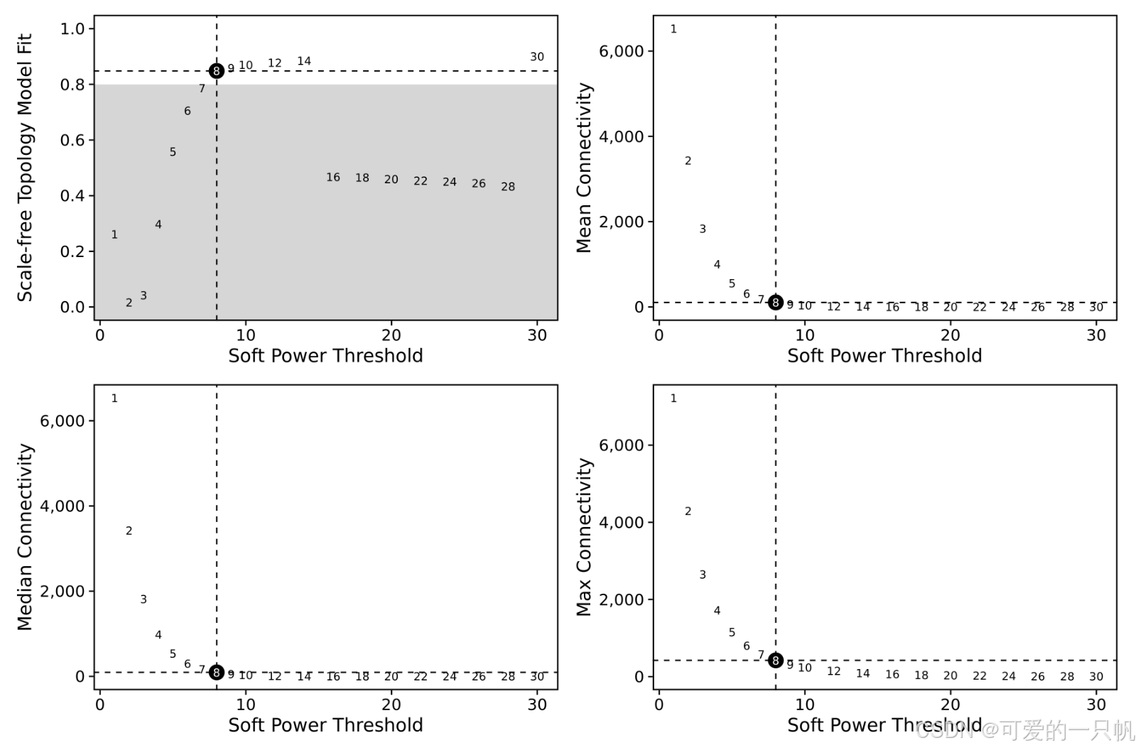
seurat_obj <- ConstructNetwork(
  seurat_obj,
  tom_name = 'INH'
)
PlotDendrogram(seurat_obj, main='INH hdWGCNA Dendrogram')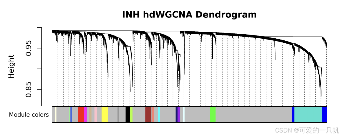
5. 计算模块特征基因
seurat_obj <- ModuleEigengenes(
 seurat_obj,
 group.by.vars="Sample"
)

hMEs <- GetMEs(seurat_obj)
MEs <- GetMEs(seurat_obj, harmonized=FALSE)
seurat_obj@misc$tutorial$wgcna_modules %>% head
6. 计算模块连接性
seurat_obj <- ModuleConnectivity(
  seurat_obj,
  group.by = 'cell_type', group_name = 'INH'
)
seurat_obj <- ResetModuleNames(
  seurat_obj,
  new_name = "INH-M"
)

p <- PlotKMEs(seurat_obj, ncol=5)
p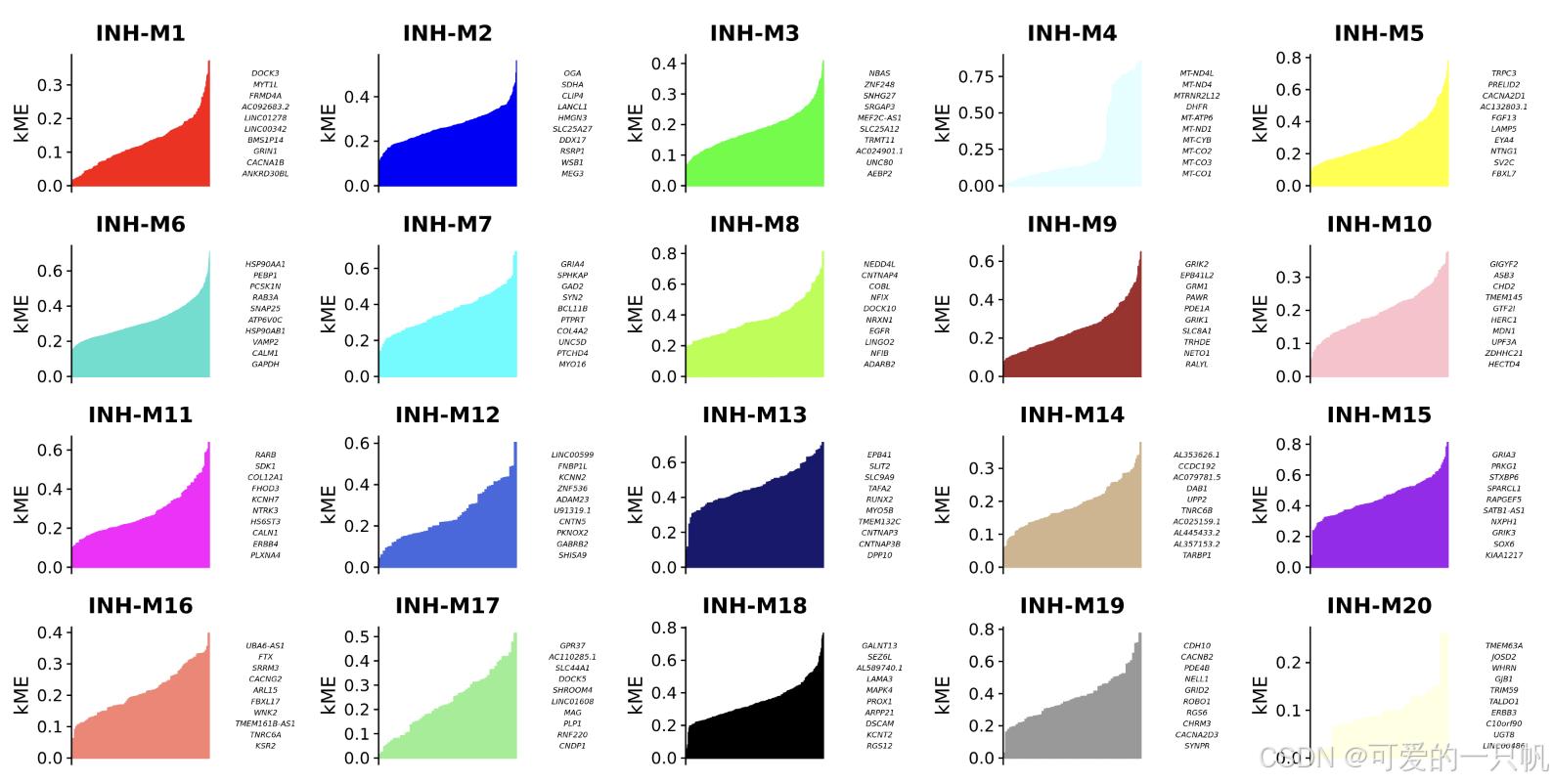
7. 获取模块分配表,提取排名靠前的hub基因
modules <- GetModules(seurat_obj) %>% subset(module != 'grey')
head(modules[,1:6])
#           gene_name module     color   kME_grey  kME_INH-M1 kME_INH-M2
# LINC01409 LINC01409 INH-M1       red 0.06422496  0.14206189 0.02146438
# INTS11       INTS11 INH-M2      blue 0.19569750  0.04996486 0.22687525
# CCNL2         CCNL2 INH-M3     green 0.21124081  0.04668528 0.20013727
# GNB1           GNB1 INH-M4 lightcyan 0.24093763  0.03203763 0.20114899
# TNFRSF14   TNFRSF14 INH-M5    yellow 0.01315166  0.02388175 0.02342308
# TPRG1L       TPRG1L INH-M6 turquoise 0.10138479 -0.05137751 0.12394048

hub_df <- GetHubGenes(seurat_obj, n_hubs = 10)
head(hub_df)
#  gene_name module       kME
# 1 ANKRD30BL INH-M1 0.3711414
# 2   CACNA1B INH-M1 0.3694937
# 3     GRIN1 INH-M1 0.3318094
# 4   BMS1P14 INH-M1 0.3304103
# 5 LINC00342 INH-M1 0.3252982
# 6 LINC01278 INH-M1 0.3100343
计算每个模块hub基因的表达活性 (module score):
library(UCell)
seurat_obj <- ModuleExprScore(
  seurat_obj,
  n_genes = 25,
  method='UCell'
)
8. 可视化
每个细胞对于每个模块的特征值:
plot_list <- ModuleFeaturePlot(
  seurat_obj,
  features='hMEs',
  order=TRUE
)
wrap_plots(plot_list, ncol=6)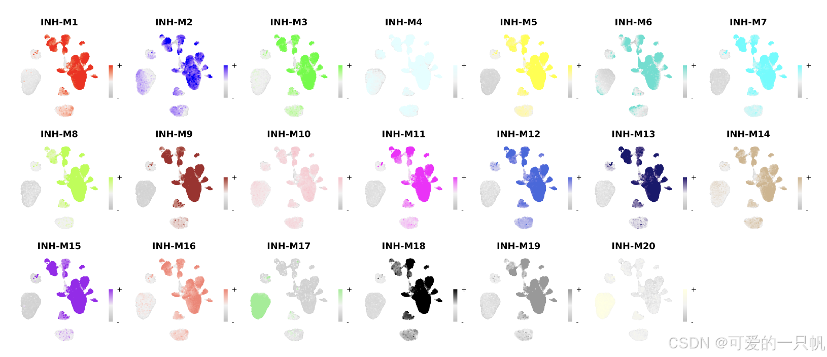
每个细胞对于每个模块hub基因的表达活性:
plot_list <- ModuleFeaturePlot(
  seurat_obj,
  features='scores',
  order='shuffle',
  ucell = TRUE
)
wrap_plots(plot_list, ncol=6)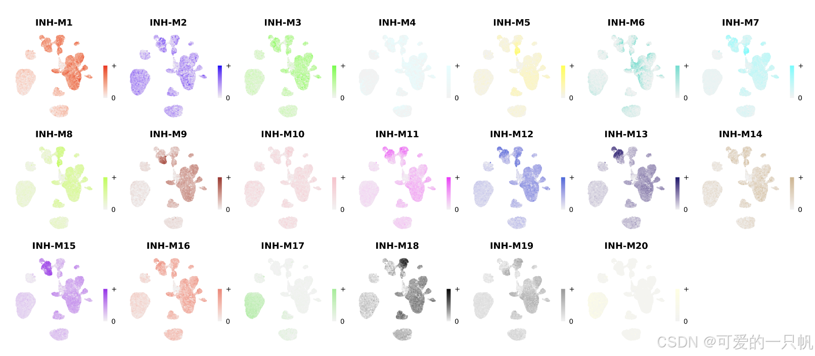
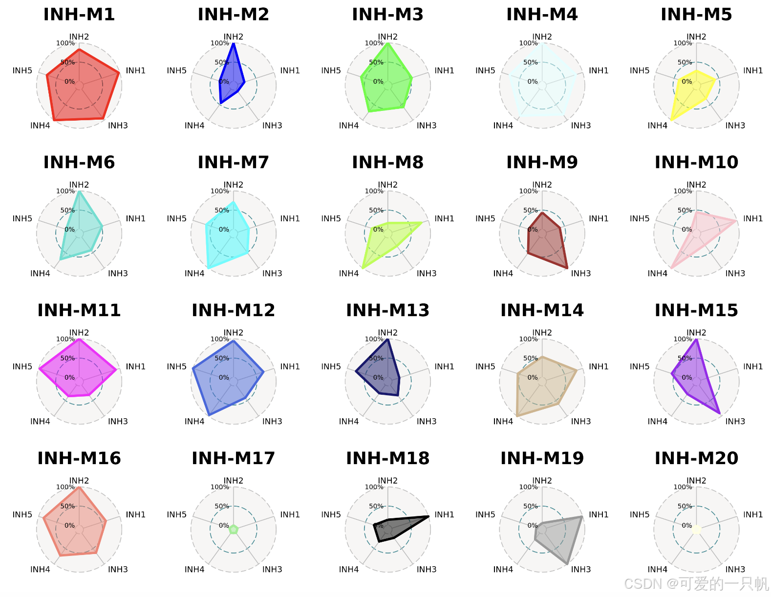
每个模块在不同分组中的相对表达水平:
seurat_obj$cluster <- do.call(rbind, strsplit(as.character(seurat_obj$annotation), ' '))[,1]

ModuleRadarPlot(
  seurat_obj,
  group.by = 'cluster',
  barcodes = seurat_obj@meta.data %>% subset(cell_type == 'INH') %>% rownames(),
  axis.label.size=4,
  grid.label.size=4
)
可视化每个模块之间的相关性:
ModuleCorrelogram(seurat_obj)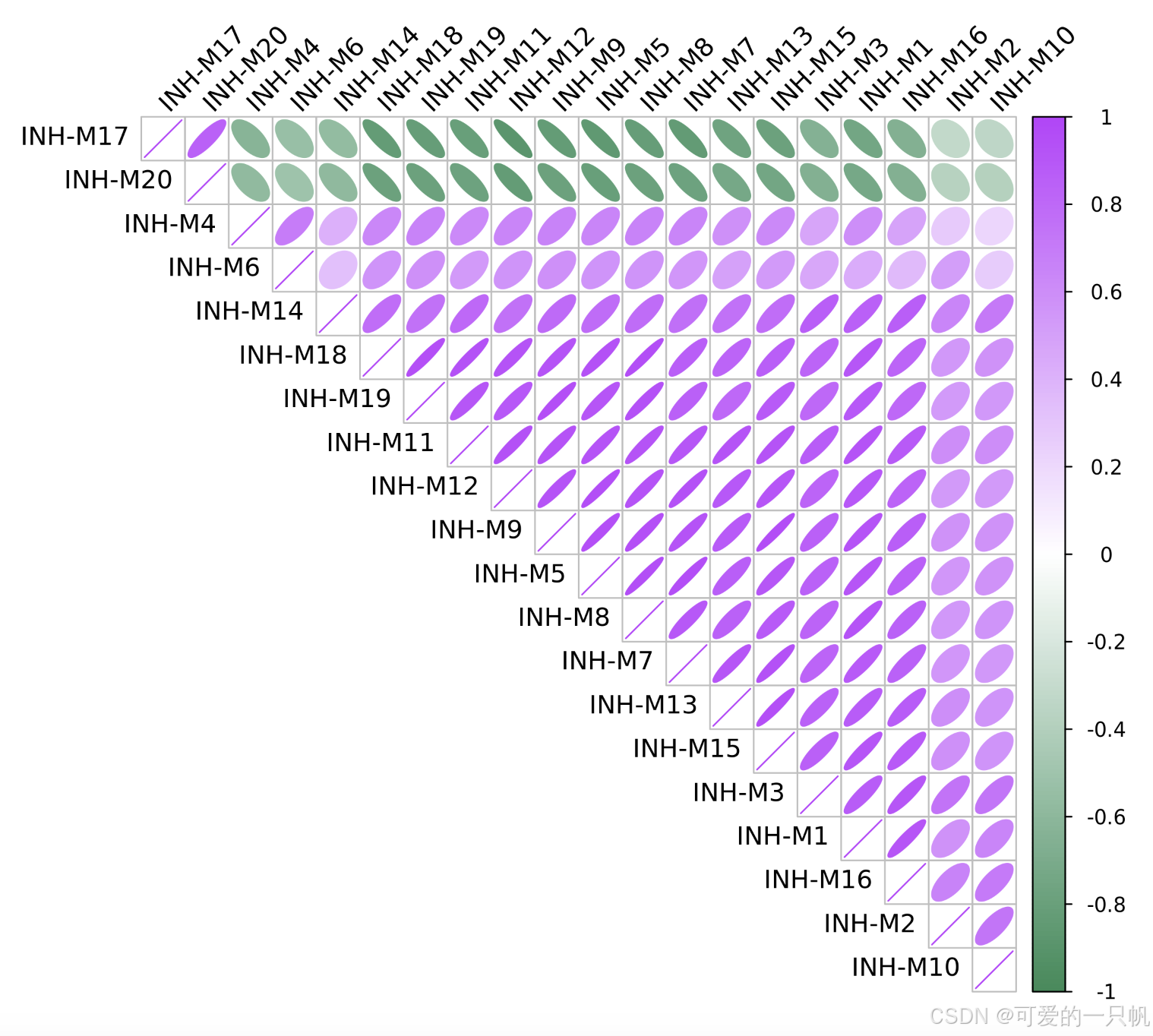
将结果加入Seurat 对象,并可视化:
MEs <- GetMEs(seurat_obj, harmonized=TRUE)
modules <- GetModules(seurat_obj)
mods <- levels(modules$module); mods <- mods[mods != 'grey']

# add hMEs to Seurat meta-data:
seurat_obj@meta.data <- cbind(seurat_obj@meta.data, MEs)

p <- DotPlot(seurat_obj, features=mods, group.by = 'cell_type')
p <- p +
  RotatedAxis() +
  scale_color_gradient2(high='red', mid='grey95', low='blue')
p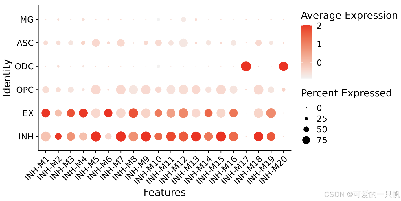
参考:hdWGCNA in single-cell data • hdWGCNA (smorabit.github.io)


 被折叠的 条评论
为什么被折叠?
被折叠的 条评论
为什么被折叠?
 到【灌水乐园】发言


