


学习来源:https://www.bilibili.com/video/BV1UJ411A7Fs(b站真是个神奇的地方……)
目录
2.Series有多层索引MultiIndex怎样筛选数据?
4.DataFrame有多层索引MultiIndex怎样筛选数据?
一、读取数据
三种格式的数据:csv、txt、mysql。
(1) csv
path = 'C:/Users/Desktop/1.csv'
a = pd.read_csv(path,encoding = 'utf-8')
(2) txt
path = 'C:/Users/Desktop/a.txt'
b = pd.read_csv(
    path,
    sep = '\t',
    header = None,
    names = ['a','b','c']
)
(3) mysql(需要先把MySQL服务器打开不然连接不上的)
import pymysql as pm
conn = pm.connect(
    user = 'root',
    password = '111',
    database = 'school'
)
s = pd.read_sql("select * from student",con = conn)
创建Series:
sq = pd.Series([1,'a',5.2,7],index = ['a','b','c','d'])
sq.index
sq.values
用字典创建:
sdata = {'a':100,'b':89,'c':20}
s2 = pd.Series(sdata)
列表多值查询:
s2[['a','b']]DataFrame读数
先创建一个df
data={
        'state':['Ohio','Ohio','Ohio','Nevada','Nevada'],
        'year':[2000,2001,2002,2001,2002],
        'pop':[1.5,1.7,3.6,2.4,2.9]
    }
df = pd.DataFrame(data)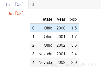
查询一行,index为列名
df.loc[1]state Ohio
year 2001
pop 1.7
Name: 1, dtype: objectdf切片包括末尾元素:
df.loc[1:3]查询
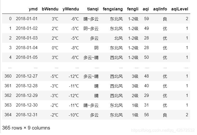
先读入一个df,后面会经常用到。
path = 'C:/Users/Desktop/a.txt'
b = pd.read_csv(
    path,
    sep = '\t',
    header = None,
    names = ['ymd','bWendu','yWendu','tianqi','fengxiang','fengli','aqi','aqiInfo','aqiLevel']
)
set_index 设置日期为索引,不创建新对象,inplace=True 修改原数据:
b.set_index('ymd',inplace = True)把摄氏度单位删去:
b.loc[:,'bWendu'] = b['bWendu'].str.replace("℃","").astype('int32')
b.loc[:,'yWendu'] = b['yWendu'].str.replace("℃","").astype('int32')
读取数据:
b.loc[['2018-01-02','2018-01-05'],['fengxiang','aqi']]可以直接按照切片读取:
b.loc['2018-01-02':'2018-01-10','fengxiang':'aqi']apply方法
def get_wendu(x):
    if x['bWendu'] > 33:
        return '高温'
    if x['yWendu'] < -10:
        return '低温'
    return '常温'
#series index 是columns
b.loc[:,"wendu_type"] = b.apply(get_wendu,axis = 1)assign方法
# 可以同时添加多个新的列
b.assign(
    yWendu_huashi = lambda x : x["yWendu"] * 9 / 5 + 32,
    # 摄氏度转华氏度
    bWendu_huashi = lambda x : x["bWendu"] * 9 / 5 + 32
)
二、数据统计函数
1.汇总
b.describe()
b['bWendu'].mean()
2.唯一去重和按值计数
b["fengxiang"].unique()
b["fengxiang"].value_counts()
3.相关系数协方差
协方差:衡量同向反向程度,如果协方差为正,说明X,Y同向变化,协方差越大说明同向程度越高;如果协方差为负,说明X,Y反向运动,协方差越小说明反向程度越高。
相关系数:衡量相似度程度,当他们的相关系数为1时,说明两个变量变化时的正向相似度最大,当相关系数为-1时,说明两个变量变化的反向相似度最大
b.cov() #协方差
b.corr()#相关系数
# 单独查看空气质量和最高温度的相关系数
b["aqi"].corr(b["bWendu"])三、缺失值
isnull和notnull:检测是否是空值,可用于df和series
dropna:丢弃、删除缺失值
- axis : 删除行还是列,0行1列, 默认0
- how : 如果等于any则任何值为空都删除,如果等于all则所有值都为空才删除
- inplace : 如果为True则修改当前df,否则返回新的df
fillna:填充空值
- value:用于填充的值,可以是单个值,或者字典(key是列名,value是值)
- method : 等于ffill使用前一个不为空的值填充forword fill;等于bfill使用后一个不为空的值填充backword fill
- axis : 按行还是列填充,0行1列
- inplace : 如果为True则修改当前df,否则返回新的df
c.dropna(axis = 'columns',how='all',inplace=True)把分数为null的填充为0
c.fillna({'分数':0})等同于:
c.loc[:,'分数'] = c['分数'].fillna(0)拿前面的填充后面的
c.loc[:,'姓名'] = c['姓名'].fillna(method='ffill') #forward fill四、settingwithcopywarning
不知道你到底是创建一个新的df还是在原来的上面修改,就会有warning。
解决办法:要么直接.loc修改原数据,要么先copy
五、数据排序
Series.sort_values(ascending=True, inplace=False)
ascending:默认为True升序排序,为False降序排序
inplace:是否修改原始Series
DataFrame.sort_values(by, ascending=True, inplace=False)
by:字符串或者List,单列排序或者多列排序
ascending:bool或者List
inplace:是否修改原始DataFrame
b['aqi'].sort_values()dataframe排序
其中如果按照多个列排序的话,可以指定哪个是降序哪个是升序。
b.sort_values(by='aqi',ascending=False)
b.sort_values(by=['aqi','bWendu'])
b.sort_values(by=['aqi','bWendu'],ascending=[True,False])
六、字符串处理
文档:https://pandas.pydata.org/pandas-docs/stable/reference/series.html#string-handling
使用方法:先获取Series的str属性,然后在属性上调用函数;
Dataframe上没有str属性和处理方法
df["bWendu"].str.replace("℃", "").astype('int32')condition = b["ymd"].str.startswith("2018-03")b['ymd'].str.replace('-','')注意:slice是str上的方法,如
b['ymd'].str.replace('-','').str.slice(0,6) 七、axis参数
d.drop('A',axis = 1) --删除某一列 axis = 1
d.drop(1,axis = 0)  --删除某一行 axis = 0
指定了行,行要动起来,列不动。【跨行输出】
制定了列,列要动起来,行不动。【跨列输出】
d.mean(axis = 0) --跨行输出八、索引index
设置索引
b.set_index('ymd',inplace=True,drop = False) -- drop false表示不删除这一列接下来就可以直接拿日期作为索引查询数据了:
b.loc['2018-01-01']九、merge
pd.merge(left, right, how='inner', on=None, left_on=None, right_on=None,
left_index=False, right_index=False, sort=True, suffixes=('_x', '_y'),
copy=True, indicator=False, validate=None)
left,right:要merge的dataframe或者有name的Series
how:join类型,'left', 'right', 'outer', 'inner'
on:join的key,left和right都需要有这个key
left_on:left的df或者series的key
right_on:right的df或者seires的key
left_index,right_index:使用index而不是普通的column做join
suffixes:两个元素的后缀,如果列有重名,自动添加后缀,默认是('_x', '_y')
和sql联结简直一模一样…
s5 =pd.merge(
    s3,s2,left_on = 's_id',right_on = 's_id',how='inner'
)
三种形式:一对一,一对多,多对多(笛卡尔积)
非key字段重名?
pd.merge(left, right, on='key')--默认加后缀
pd.merge(left, right, on='key', suffixes=('_left', '_right'))--自己定义
十、concat
pandas.concat(objs, axis=0, join='outer', ignore_index=False)
objs:一个列表,内容可以是DataFrame或者Series,可以混合
axis:默认是0代表按行合并,如果等于1代表按列合并
join:合并的时候索引的对齐方式,默认是outer join,也可以是inner join
ignore_index:是否忽略掉原来的数据索引
DataFrame.append(other, ignore_index=False)
append只有按行合并,没有按列合并,相当于concat按行的简写形式
other:单个dataframe、series、dict,或者列表
ignore_index:是否忽略掉原来的数据索引
pd.concat([df1,df2]) --默认axis=0,join=outer,ingnore_index=false
pd.concat([df1,df2],ignore_index=True)--原来的数字索引忽略了,现在给出了新的数字索引
pd.concat([df1,df2],ignore_index=True,join="inner")
pd.concat([df1,s1,s2],axis=1)
用append按行合并
df1.append(df2)
df1.append(df2,ignore_index=True)--原来的数字索引忽略了,现在给出了新的数字索引
十一、分组统计groupby
例表:
df = pd.DataFrame({'A': ['foo', 'bar', 'foo', 'bar', 'foo', 'bar', 'foo', 'foo'],
                   'B': ['one', 'one', 'two', 'three', 'two', 'two', 'one', 'three'],
                   'C': np.random.randn(8),
                   'D': np.random.randn(8)})
df| A | B | C | D | |
| 0 | foo | one | 1.523523 | -0.687054 |
| 1 | bar | one | 1.545824 | 0.622031 |
| 2 | foo | two | -0.024231 | 0.387469 |
| 3 | bar | three | -1.794833 | 0.297639 |
| 4 | foo | two | 1.860476 | -0.205438 |
| 5 | bar | two | 0.207021 | -0.929341 |
| 6 | foo | one | 1.055254 | -0.685854 |
| 7 | foo | three | -0.349821 | -0.501275 |
对A分组,分别求和:
df.groupby('A').sum()对AB分组:
df.groupby(['A','B']).mean()df.groupby(['A','B'],as_index=False).mean()计算多种聚合:
df.groupby('A').agg([np.sum, np.mean, np.std])单列结果数据统计:
df.groupby('A')['C'].agg([np.sum, np.mean, np.std])分别统计:
df.groupby('A').agg({"C":np.sum, "D":np.mean})获取单个分组的数据:
g = df.groupby('A')
g.get_group('bar')

g = df.groupby(['A', 'B'])
g.get_group(('foo', 'two'))
十二、分层索引MultiIndex
多维索引分层查看
1.Series的分层索引MultiIndex
aa = b.groupby(['fengli','tianqi'])['aqi'].min()
aa.index
MultiIndex([('1-2级', '中雨~小雨'),
('1-2级', '中雨~雷阵雨'),
('1-2级', '多云'),
('1-2级', '多云~小雨'),
('1-2级', '多云~晴'),
('1-2级', '多云~阴'),
('1-2级', '多云~雷阵雨'),
('1-2级', '小雨'),……unstack把二级索引变成列:
aa.unstack()2.Series有多层索引MultiIndex怎样筛选数据?
aa.loc['4-5级']tianqi
多云 22
多云~小雨 164
多云~晴 21
晴 25
Name: aqi, dtype: int64多层索引-元组:
aa.loc[('4-5级','多云~小雨')]第一层全部,第二层……:
aa.loc[:,'多云~晴'] 3.DataFrame的多层索引MultiIndex
设置索引:
bb = b.set_index(['tianqi','fengxiang'])
bb.index
MultiIndex([('晴~多云', '东北风'),
('阴~多云', '东北风'),
( '多云', '北风'),
( '阴', '东北风'),
('多云~晴', '西北风'),
('多云~阴', '西南风'),
('阴~多云', '西南风'),
( '晴', '西北风'),……4.DataFrame有多层索引MultiIndex怎样筛选数据?
元组(key1,key2)代表筛选多层索引,其中key1是索引第一级,key2是第二级
列表[key1,key2]代表同一层的多个KEY,其中key1和key2是并列的同级索引
bb.loc[('中雨~雷阵雨','南风')]
bb.loc[('中雨~雷阵雨','南风'),'ymd']
bb.loc[['中雨~雷阵雨','霾'],:]

# slice(None)代表筛选这一索引的所有内容
bb.loc[(slice(None), ['东南风', '西风']), :]
将索引重新转换为列:是set_index的逆操作
reset_index()十三、数据转换函数map、apply、applymap
1. map用于Series值的转换
数据转换函数对比:map、apply、applymap:
map:只用于Series,实现每个值->值的映射;
apply:用于Series实现每个值的处理,用于Dataframe实现某个轴的Series的处理;
applymap:只能用于DataFrame,用于处理该DataFrame的每个元素;
#映射
fengxiang_names = {
    '东北风':'northeast',
    '北风':'north',
    '西北风':'northwest',
    '西南风':'Southwest',
    '南风':'south',
    '东南风':'southeast',
    '东风':'east',
    '西风':'west'
}
方法1:Series.map(dict)
b['风向'] = b['fengxiang'].map(fengxiang_names)方法2:Series.map(function)
function的参数是Series的每个元素的值
b['风向1'] = b['fengxiang'].map(lambda x:fengxiang_names[x])2. apply用于Series和DataFrame的转换
Series.apply(function), 函数的参数是每个值
DataFrame.apply(function), 函数的参数是Series
b['风向2'] = b['fengxiang'].apply(lambda x:fengxiang_names[x])b['风向3']=b.apply(lambda x:fengxiang_names[x['fengxiang']],axis=1)(lambda x的x是一个Series,因为指定了axis=1所以Seires的key是列名,可以用x['fengxiang']获取)
3. applymap用于DataFrame所有值的转换
cc = b[['bWendu','aqi','yWendu']]
cc.applymap(lambda x:abs(x))
直接赋值给原表:
b.loc[:,['bWendu','aqi','yWendu']] = cc.applymap(lambda x:abs(x))以上。其余的画图啊什么的内容下次再总结吧。(下次一定)
---END---


 747
747

 被折叠的 条评论
为什么被折叠?
被折叠的 条评论
为什么被折叠?
 到【灌水乐园】发言


