线性回归

使用jupyter notebook实现，python3语法

#%%

#导入包
import numpy as np
import matplotlib.pyplot as plt
import pandas as pd

#%%

# 导入数据
datafile = 'ex1data1.txt'
cols = np.loadtxt(datafile,delimiter=',',unpack=True,usecols=(0,1))
X = np.transpose(np.array(cols[:-1]))
y = np.transpose(np.array(cols[-1:]))
m = y.size
X = np.insert(X,0,1,axis=1)
print(X.shape[1])

输出结果：2

#%%

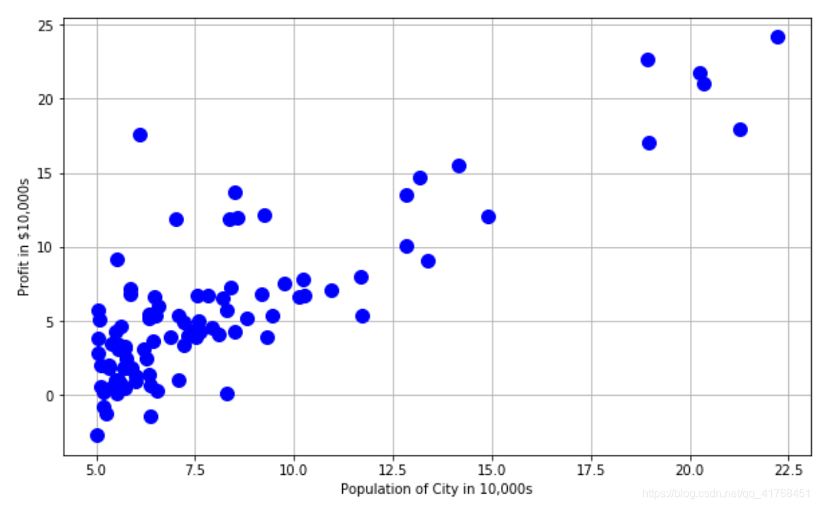
# 绘图
plt.figure(figsize=(10,6))
plt.plot(X[:,1],y[:,0],'bo',markersize = 10)
plt.grid(True)
plt.ylabel('Profit in $10,000s')
plt.xlabel('Population of City in 10,000s')

#%%

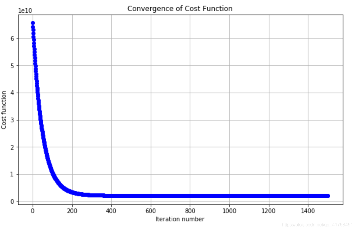
iterations = 1500 # 迭代次数
alpha = 0.01 # 步长


#%%

# 预测函数
def h(theta,X):
    return np.dot(X,theta)

# 损失函数
def computeCost(theta,X,y):
    return float(1/(2*m)*np.dot(np.transpose((h(theta,X)-y)),(h(theta,X)-y)))

mytheta = np.zeros((X.shape[1],1))
print(computeCost(mytheta,X,y))

输出结果：32.072733877455676

#%%

# 梯度下降函数
def grandientDescent(X,y,theta = np.zeros(2)):
    cost = []
    thetahistory = []
    for iteration in range(iterations):
        tmptheta = theta
        cost.append(computeCost(theta,X,y))
        thetahistory.append(list(theta[:,0]))
        for j in range(len(tmptheta)):
            tmptheta[j] = theta[j] - (alpha/m)*np.sum((h(theta,X) - y)*np.array(X[:,j]).reshape(m,1))
        theta = tmptheta
    return theta,thetahistory,cost
    
    


#%%

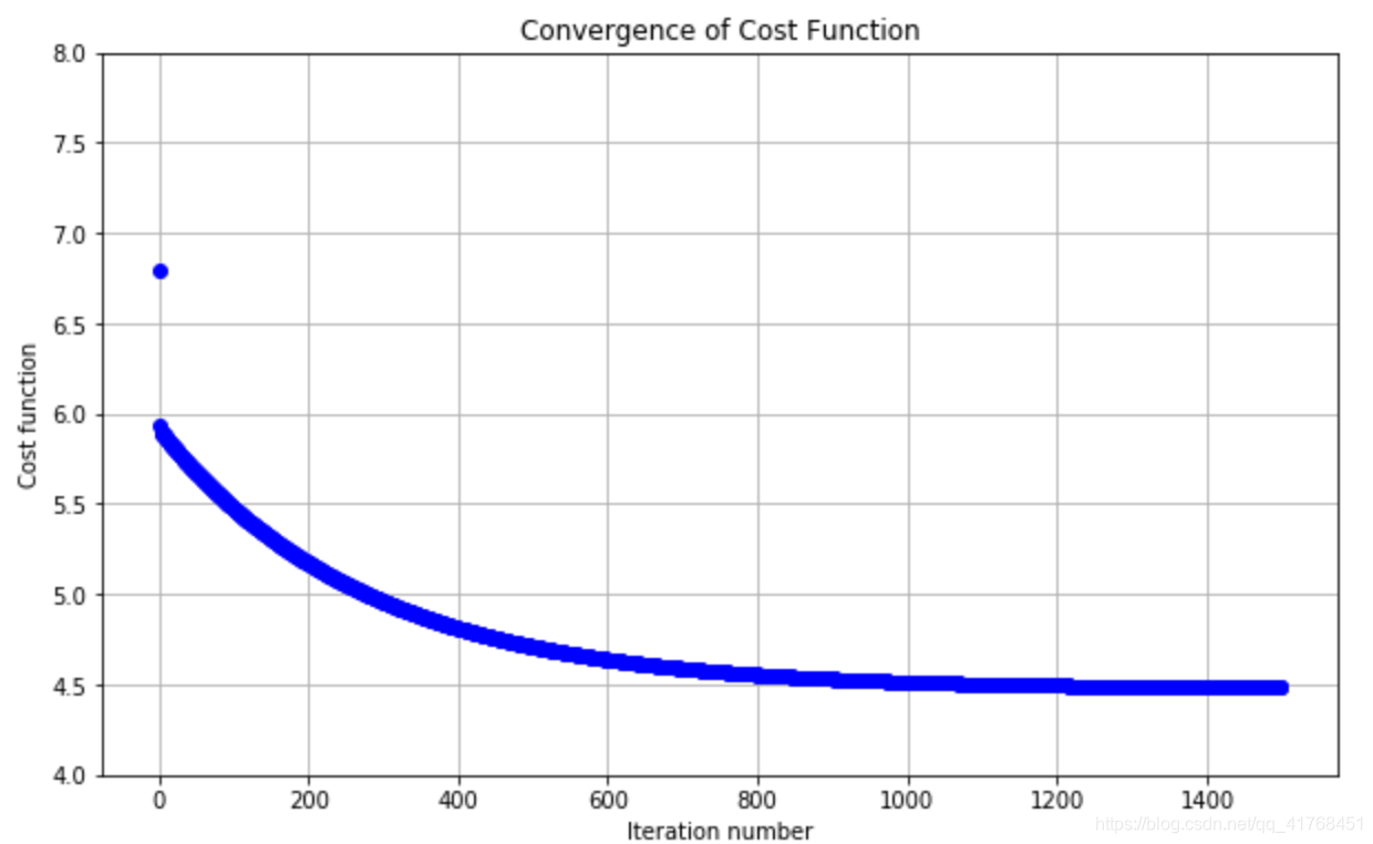
theta,thetahistory,cost = grandientDescent(X,y,mytheta)
def plotConvergence(cost):
    plt.figure(figsize=(10,6))
    plt.plot(range(len(cost)),cost,'bo')
    plt.grid(True)
    plt.title("Convergence of Cost Function")
    plt.xlabel("Iteration number")
    plt.ylabel("Cost function")
    plt.xlim(-0.05*iterations,1.05*iterations)
    plt.ylim(4,8)  
plotConvergence(cost)

#%%

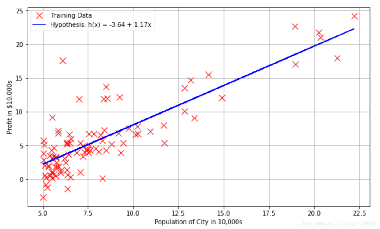
# 绘制拟合后得到的曲线
def myfit(xval):
    return theta[0] + theta[1]*xval

plt.figure(figsize=(10,6))
plt.plot(X[:,1],y[:,0],'rx',markersize=10,label='Training Data')
plt.plot(X[:,1],myfit(X[:,1]),'b-',label = 'Hypothesis: h(x) = %0.2f + %0.2fx'%(theta[0],theta[1]))
plt.grid(True) 
plt.ylabel('Profit in $10,000s')
plt.xlabel('Population of City in 10,000s')
plt.legend()

#%%

from mpl_toolkits.mplot3d import axes3d, Axes3D
from matplotlib import cm
import itertools

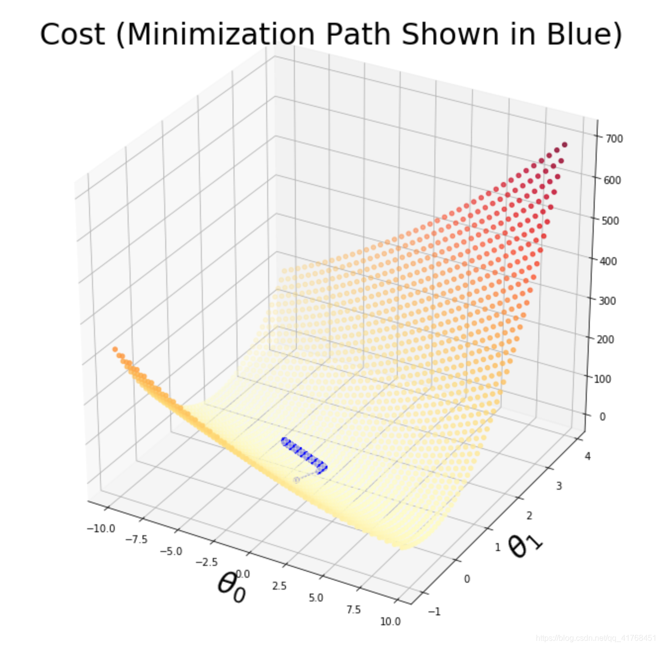
fig = plt.figure(figsize=(12,12))
ax = fig.gca(projection='3d')

xvals = np.arange(-10,10,.5)
yvals = np.arange(-1,4,.1)
myxs, myys, myzs = [], [], []
for david in xvals:
    for kaleko in yvals:
        myxs.append(david)
        myys.append(kaleko)
        myzs.append(computeCost(np.array([[david], [kaleko]]),X,y))

scat = ax.scatter(myxs,myys,myzs,c=np.abs(myzs),cmap=plt.get_cmap('YlOrRd'))

plt.xlabel(r'$\theta_0$',fontsize=30)
plt.ylabel(r'$\theta_1$',fontsize=30)
plt.title('Cost (Minimization Path Shown in Blue)',fontsize=30)
plt.plot([x[0] for x in thetahistory],[x[1] for x in thetahistory],cost,'bo-')
plt.show()

#%%

#  多变量线性回归
datafile2 = 'ex1data2.txt'
cols2 = np.loadtxt(datafile2,delimiter=',',unpack=True,usecols=(0,1,2))
X2 = np.transpose(np.array(cols2[:-1]))
y2 = np.transpose(np.array(cols2[-1:]))
m = y2.size
X2 = np.insert(X2,0,1,axis=1)

#%%

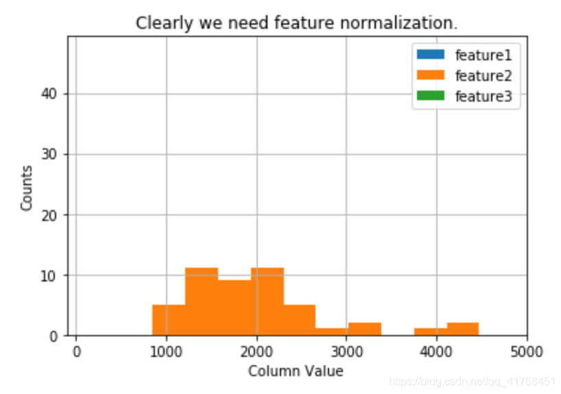
# 绘图
plt.grid(True)
plt.xlim([-100,5000])
plt.hist(X2[:,0],label = 'feature1')
plt.hist(X2[:,1],label = 'feature2')
plt.hist(X2[:,2],label = 'feature3')
plt.title('Clearly we need feature normalization.')
plt.xlabel('Column Value')
plt.ylabel('Counts')
plt.legend()

#%%

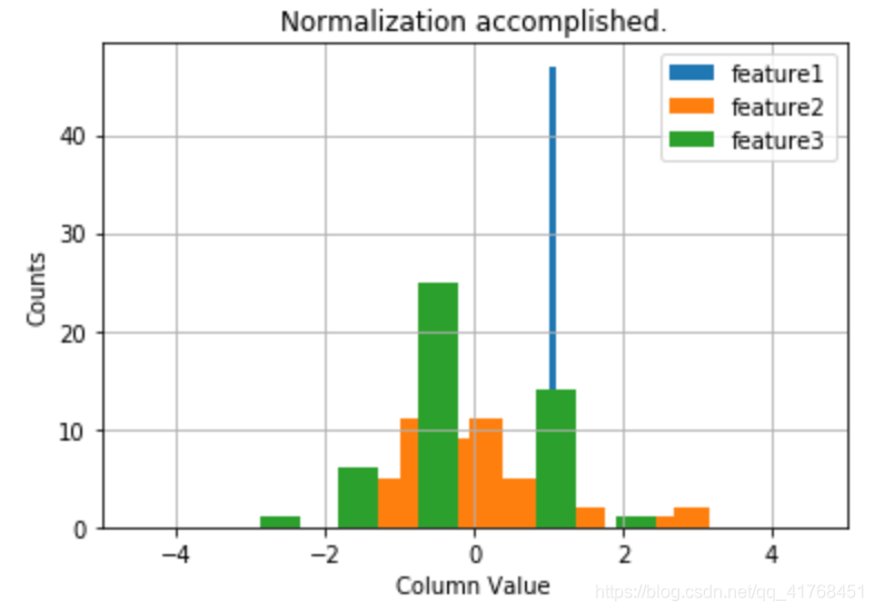
# 对数据规范化
stored_feature_means,stored_feature_stds = [],[]
X2norm = X2.copy()
print(X2norm.shape[1])
for col in range(X2norm.shape[1]):
     stored_feature_means.append(np.mean(X2norm[:,col]))
     stored_feature_stds.append(np.std(X2norm[:,col]))
    
     if not col: continue
     X2norm[:,col] = (X2norm[:,col] - stored_feature_means[-1])/stored_feature_stds[-1]

#%%

plt.grid(True)
plt.xlim([-5,5])
plt.hist(X2norm[:,0],label = 'feature1')
plt.hist(X2norm[:,1],label = 'feature2')
plt.hist(X2norm[:,2],label = 'feature3')
plt.title('Normalization accomplished.')
plt.xlabel('Column Value')
plt.ylabel('Counts')
plt.legend()

#%%

# 梯度下降
mytheta2 = np.zeros((X2norm.shape[1],1))
theta, thetahistory, cost2 = grandientDescent(X2norm,y2,mytheta2)
def plotConvergence2(cost):
    plt.figure(figsize=(10,6))
    plt.plot(range(len(cost)),cost,'bo')
    plt.grid(True)
    plt.title("Convergence of Cost Function")
    plt.xlabel("Iteration number")
    plt.ylabel("Cost function")
    plt.xlim(-0.05*iterations,1.05*iterations)
plotConvergence2(cost2)

#%%

ytest = np.array([1.,1650.,3.])

# for  i in range(len(ytest)):
ytestnorm = (ytest - stored_feature_means) / stored_feature_stds

ytestnorm[0] = 1
print ("$ %0.2f" % float(h(mytheta2,ytestnorm)))

输出结果：
$ 293098.15

#%%

# 解析法求解
from numpy.linalg import inv
def normEqtn(X,y):
    return np.dot(np.dot(inv(np.dot(X.T,X)),X.T),y)


print ("$%0.2f" % float(h(normEqtn(X2,y2),[1,1650.,3])))

输出结果：
$293081.46