close all
clear
clc
% 定义时间变量
t = 0:0.01:10; % 从0到10,步长为0.01
% 定义不同的频率和相位
f1 = 0.5;
f2 = 1;
f3 = 2;
phi1 = 0;
phi2 = pi/4;
phi3 = pi/6;
% 添加一个线性趋势
linear_trend = 0.2 * t;
% 添加噪声
noise = 0.1 * randn(size(t));
% 生成复杂的合成信号
x = sin(2 * pi * f1 * t + phi1) + 0.5 * cos(2 * pi * f2 * t + phi2) + 0.3 * sin(2 * pi * f3 * t + phi3) + linear_trend + noise;
% 获取不同时间下的数据自相关系数
Rxtemp = [];
for k=1:length(t)
R_xx = max(xcorr(x(1,1:k)))/(k*2);
Rxtemp = [Rxtemp R_xx];
end
figure;
plot(Rxtemp)
% n为显示分量个数
n =8;
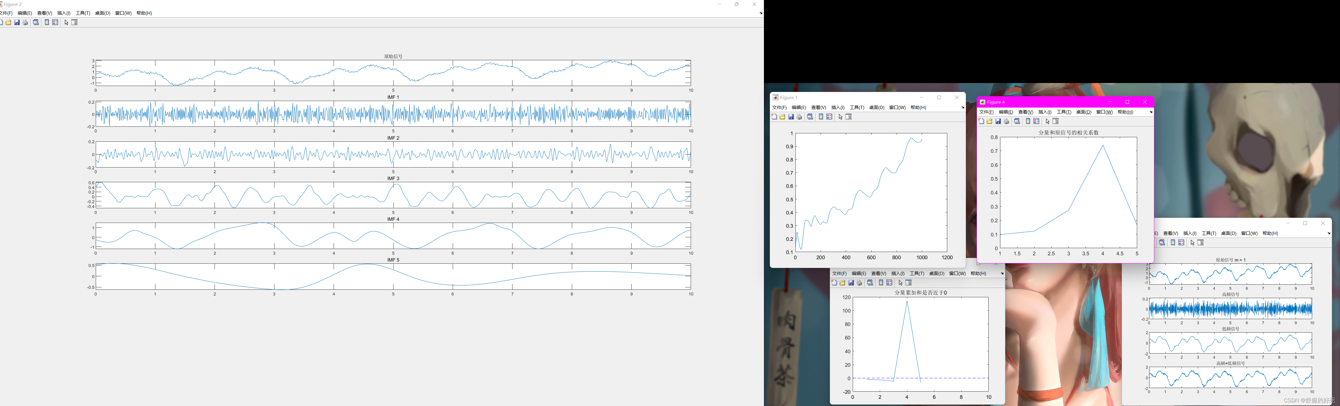
% 绘制原始信号
figure;
subplot(n, 1, 1);
plot(t, x);
title('原始信号');
% 使用EMD函数进行分解
imf = emd(x);
temp=[];
Rtemp =[];
% 显示IMFs
for k = 1:size(imf, 2)
subplot(n ,1, k + 1);
plot(t, imf(:, k));
%分量累加和是否近于0
temp = [temp sum(imf(:,k))];
%分量和原信号的相关系数
R = corrcoef(x, imf(:,k));
Rtemp = [Rtemp R(1,2)];
title(['IMF ', num2str(k)]);
end
figure;
plot(temp)
hold on
plot(t,zeros(1,length(t)),'b--')
title('分量累加和是否近于0')
figure;
plot(Rtemp)
title('分量和原信号的相关系数')
%m为高低频分界分量,m以上为高频信号重构(不包括m),m以下为低频信号重构(包括m)
m=1;
% 绘制重构信号
figure;
subplot(4, 1, 1);
plot(t, x);
title('原始信号 m = '+string(m));
subplot(4, 1, 2);
plot(t, sum(imf(:,1:m)', 1));
title('高频信号');
subplot(4, 1, 3);
plot(t, sum(imf(:,m+1:end)', 1));
title('低频信号');
subplot(4, 1, 4);
plot(t, sum(imf(:,1:m)', 1)+sum(imf(:,m+1:end)', 1));
title('高频+低频信号');


 1080
1080

 被折叠的 条评论
为什么被折叠?
被折叠的 条评论
为什么被折叠?
 到【灌水乐园】发言


