[paper reading] YOLO v1

[paper reading] YOLO v1

GitHub：Notes of Classic Detection Papers

本来想放到GitHub的，结果GitHub不支持公式。
没办法只能放到优快云，但是格式也有些乱
强烈建议去GitHub上下载源文件，来阅读学习！！！这样阅读体验才是最好的
当然，如果有用，希望能给个star！

topic	motivation	technique	key element	use yourself	relative
YOLO v1	Problem to Solve Detection as Regression	YOLO v1 Architecture	Grid Partition Model Output “Responsible” NMS Getting Detections Error Type Analysis Handle Small Object Data Augmentation	Classification & Detection Explicit & Implicit Grid Multi-Task Output Loss & Sample & box NMS Data Augmentation	Articles Code Blogs

Motivation

Problem to Solve

two-stage的方法本质上是使用classification进行detection，而导致无法直接优化detection的性能

Detection as Regression

将object detection归为regression问题，从而在空间上分离 bounding boxes 和 class probability

使用单个网络，对full image进行一次evaluation，得到bounding box和class probability，从而直接优化detection的表现

Technique

YOLO v1 Architecture

YOLO的最后一层采用线性激活函数，其它层都是Leaky ReLU。

训练的时候使用小图片（224×225），测试的时候使用大图片（448×448）

Essence

使用一个CNN实现以下功能：

• feature extraction ==> 卷积层（backbone） ==> contextual reasoning
• prediction
  • bounding box prediction
  • classification
• non-maximum suppression ==> post-processing

Steps

1. resize image to fixed size
2. CNN ==> feature extraction & classification
3. Non-max suppression ==> post-process

实验中detection相关参数含义如下：

• $S$ ：将resized image划分为 $S\times S$ 个 grid

  实验中设置为 7

• $B$ ：每个 grid 预测的 bounding box 的数目

  实验中设置为 2

• $C$ ：实验中目标的类别数

  实验中为 20

Pros

1. Unified

2. Fast

   原因：将Detection作为Regression，不需要复杂的pipeline

3. reason globally ==> 体现在feature extraction上

   在训练和测试时使用整个image，可以 implicitly encodes 关于classes和appearance的上下文信息（contextual information）

   ==> YOLO 会出现更少的 background error

4. generalizable representation

   YOLO 可以学到object的概括表示，使其在new domain和unexpected input上表现更好

   因为YOLO是从数据中学习bounding box的scale和ratios，而不是根据任务去单独设计anchor

5. Loss Function Directly to Detection Performance

   直接在detection performance上设定损失函数，可以train jointly

Cons

1. 对bbox prediction的强空间限制

   每个grid只能有2个bbox、1个class

2. 难以检测成群的small object

   详见 [Handle Small Object](#Handle Small Object)

3. 更多的 Localization 错误

   详见 [Error Type Analysis](#Error Type Analysis)

4. 难以推广到新的（或罕见的）ratios或configuration

   bbox是从数据中学习到的，而不是anchor这种预定义的scale和ratios

   详见 “Responsible” 的 Result

5. 使用了较粗的feature去预测bounding box

   因为经历了多次下采样

6. 损失函数中将big/small object同等看待

   而small object的微小误差也会对IoU产生大影响

Key Element

Grid Partition

将resized image划分为 $S\times S$ 个 grid（$S$ 是人为设定的超参数）

object的中心落在哪个grid，则对应grid负责对该目标的detection（即这个cell中confidence $\mathrm{Pr}\left({\text{ Class }}_i\mid \text{ Object }\right)$ 为1，其他cell的为0 ）

Model Output

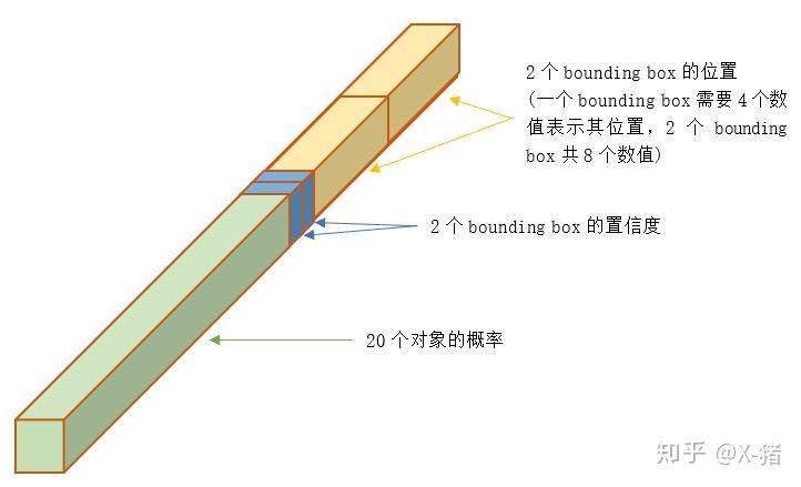
整个图片经过YOLO的输出，是一个 $S\times S\times (B\ast 5+C)$ 的 tensor（$5$ 包括 $x,y,w,h,c$）

对于每一个单元格，前20个元素是类别概率值class probability，然后2个元素是边界框置信度confidence，两者相乘可以得到类别置信度class-specific confidence score，最后8个元素是边界框boxes的 $(x,y,w,h)$

对所有的单元格：

• Bounding Box ==> $B\ast 5$

  每个grid会预测 $B$ 个 bounding box（$B$ 个predictor），每个 bounding box 会对应5个输出：

  • bounding box location $x,y,w,h$

    $x,y$ 表示 bbox 的中心坐标（相对于cell的左上角，被cell的宽高Normalization），$w,h$ 为bbox的高和宽（被图片的高和宽Normalization）

    ==> 所以 $x,y,w,h$ 都是在 [0, 1] 之间的值

    我们通常做回归问题的时候都会将输出进行归一化，否则可能导致各个输出维度的取值范围差别很大，进而导致训练的时候，网络更关注数值大的维度。因为数值大的维度，算loss相应会比较大，为了让这个loss减小，那么网络就会尽量学习让这个维度loss变小，最终导致区别对待。

  • Confidence $c$

    表示了：

    1. box中包含object的可能性
    2. box位置的精准度

    $$\mathrm{Pr}(\text{ Object })\ast {\mathrm{I}\mathrm{O}\mathrm{U}}_{\text{pred }}^{\text{truth }}$$

    • 训练时：

      如果cell中出现object，则 $\mathrm{Pr}(\text{ Object })=1$

      如果cell中不出现object，则 $\mathrm{Pr}(\text{ Object })=0$

    • 测试时：

      网络直接输出 $\mathrm{Pr}(\text{ Object })\ast {\mathrm{I}\mathrm{O}\mathrm{U}}_{\text{pred }}^{\text{truth }}$

      需要说明：虽然有时说"预测"的bounding box，但这个IOU是在训练阶段计算的。等到了测试阶段（Inference），这时并不知道真实对象在哪里，只能完全依赖于网络的输出，这时已经不需要（也无法）计算IOU了。

• Conditional Class Probability ==> $C$

  表示bbox中有object的条件下，object为每个类别的概率
  $$\mathrm{Pr}\left({\text{ Class }}_i\mid \text{ Object }\right)$$

  注意：每个grid cell只预测一组（$C$ 维）class probability（与 $B$ 的值无关）

  • 训练时：

    如果cell中出现object，则条件满足

    如果cell中不出现object，则条件不满足

  • 测试时：

    将conditional class probabilities和box confidence predictions相乘，以获得每个box的 class-specific confidence scores
    $$\mathrm{Pr}\left({\text{ Class }}_i\mid \text{ Object }\right)\ast \mathrm{Pr}(\text{ Object })\ast {\mathrm{I}\mathrm{O}\mathrm{U}}_{\text{pred }}^{\text{truth }}=\mathrm{Pr}\left({\text{ Class }}_i\right)\ast {\mathrm{I}\mathrm{O}\mathrm{U}}_{\text{pred }}^{\text{truth }}$$
    

    

    

    为什么这么做呢？

    举个例子，对于某个cell来说，在测试阶段，即使这个cell不存在物体（即confidence的值为0），也存在一种可能：输出的条件概率 $\mathrm{Pr}\left({\text{ Class }}_i\mid \text{ Object }\right)=0.9$。

    但将 confidence 和 $\mathrm{Pr}\left({\text{ Class }}_i\mid \text{ Object }\right)$ 相乘就变为0了。这个是很合理的，因为你得确保cell中有物体（即confidence大），算类别概率才有意义。

• 对应类别在bbox中出现的概率

• bbox对object的符合程度

最后一层有2个输出：

• class probability
• bounding box coordinate

“Responsible”

Introduction

是 Object & Predictor Responsible

尽管每个 cell 有 $B$ 个predictor（预测 $B$ 个bbox），但我们希望每个predictor仅对应1个object

Implement

预测结果与ground-truth box具有最高IOU的predictor（预测box）对该object负责。

==> 相当于使用 $B$ 个predictor，最后去优化的只有“responsible”的predictor

Result

bbox predictor 的专业化

==> 每个predictor专注于特定size、ratios、class的object

NMS

Purpose

解决 multiple detections 的问题

在 YOLO 中有两类object会产生 multiple detections 的问题：

• large object（大目标）
• object near the border（靠近grid边界的目标）

Steps

• 取各个类别中置信度最高的框为第一个框（先类别）

• 设定IOU阈值，将 ==> 得到第一个目标的框

• 重复上述2步，直到没有剩余的框

Getting Detections

得到 $S\times S\times B$ 个预测的bbox后，有2种执行NMS的方法：

1. 先类别，后NMS

   • 对每个预测box，取其最高置信度的类别作为其分类类别（先类别）

   • 设置置信度阈值，过滤掉置信度较小的预测box

   • NMS去剔除多余的预测box（后NMS）（为剔除操作）

   关于对预测box一视同仁，还是根据类别来区别处理：

   其实应该根据类别区别处理，但是一视同仁也没问题，因为不同类别的目标出现在相同位置的概率很小，

2. 先NMS，后类别（YOLO采用这种方式）

   • 设置置信度阈值，过滤掉置信度较小的预测box
   • NMS将多余的预测box的置信度值归为0（先NMS）（置信度归0，非剔除）
   • 确定各个box的类别，置信度值不为0时才输出检测结果

   

Error Type Analysis

Error Type

detection的结果可以分为以下情况：

• **Correct **：correct class 且 IOU > 0.5
• Localization ：correct class 且 0.1 < IOU < 0.5
• Similar ：class is similar 且 IOU >0.1
• Other ：class is wrong 且 IOU > 0.1
• Background ：IOU <0.1 for any object

Results

YOLO产生更多的localization错误，更少的background错误 ==> 主要的错误来源是 incorrect localization

Compared to state-of-the-art detection systems, YOLO makes more localization errors but is less likely to predict false positives on background.

Our main source of error is incorrect localizations.

Reason of Localization

Localization的唯一原因就是 IOU过低，也就是bounding box的位置不对

YOLO没有像 anchor-based method 使用anchor，导致其对bounding box的学习几乎是从0开始的（anchor的翻译一般为“锚”，也就是给出bounding box的基准）。

正是因为bounding box的学习缺少了基准，导致了IOU过低，即 Localization

这个跟ResNet的shortcut connection提供基准的思想很像，都是有了基准后更容易学习和优化

Handle Small Object

YOLO中使用 $\sqrt{w_i}$ 和 $\sqrt{h_i}$ 的方法仅仅是缓解，既不是治标，更不是治本

YOLO小目标检测的问题根本原因是：在high-level的feature map中，小目标的细节信息基本全部丢失了

后续的SSD通过 multi-scale feature map 大幅度解决了这个问题

Data Augmentation

1. random scaling and translation ==> 随机缩放和平移

   随机缩放和平移的上限为原始图像尺寸的20%

   we introduce random scaling and translations of up to 20% of the original image size

2. randomly adjust the exposure and saturation ==> 随机调整曝光度和饱和度

   随机调整曝光度和饱和度的调整上限为1.5倍

   We also randomly adjust the exposure and saturation of the image by up to a factor of 1.5 in the HSV color space.

Use Yourself

Classification & Detection

一般来说，绝大多数任务都可以被视为分类问题或回归问题

无论是分类，还是回归，其输出都是向量，这意味着二者在某些条件下是可以等效的（当然需要单独设计结构）

Explicit & Implicit Grid

原图必定会以一定的步长被划分为grid。其所得的grid cell即为detection的最小单位（预测bbox的最小单位）

grid划分方式主要有两种：

• Explicit Grid

  YOLO是显性的grid划分

  • YOLO直接设定超参数 $S$ 为划分的步长，将图像划分为 $S\times S$ 的grid，每个cell的大小为 $\lfloor \frac{w}{S}\rfloor \times \lfloor \frac{h}{S}\rfloor$

  • 每个cell放置 $B$ 个predictor（bounding box）

  • 输出结果的一个像素对应一个 $\lfloor \frac{w}{S}\rfloor \times \lfloor \frac{h}{S}\rfloor$ 的cell（每个cell一定严格相邻）

• Implicit Grid

  Faster-RCNN是隐性的grid划分

  • Faster-RCNN的划分步长与backbone的下采样次数 $n$ 的关系为 $S=2^n$

  • feature map的每个点会放置一组预定义的anchor

  • feature map的一个像素对应一个 $2^n × 2^n $ 的cell（每个grid并不一定样相邻，可能有重叠或间隔）

Multi-Task Output

1个模型的输出可以包括多个Task的成分，实现不同的Task

比如YOLO中的：

• classification prediction
• bounding box prediction
• confidence

Loss & Sample & box

Sample Box Reluctant

现阶段检测的方法，实质上属于饱和式检测

其“饱和”主要体现在2点：

• 空间位置的饱和 ==> sample ==> 正/负样本（前景/背景，有目标/无目标）

  即便是YOLO仅仅将空间分为 $7\times 7$ 的grid，其cell也远远多于object ==> 负样本（背景/无目标）远远多于正样本（前景/有目标）

• bounding box的饱和 ==> box ==> “responsible” or not

  YOLO中1个cell会有 $2$ 个预测的bounding box（最后只选取1个为responsible）

  Faster-RCNN更甚，对feature map的每个点放置 $3\times 3=9$ 个anchor，但其并没有对box进行筛选

Weighted Task

对于多任务的损失，需要设定其相互的权重，才能保证可以同时对多任务优化

Loss Function & Processing

总结一下：

1. two-stage的本质是分类，stage-1仅仅是尽可能多的输出正样本

2. two-stage在面对饱和式检测导致的正负样本不平衡中，由于stage-1的存在，而具有天然的优势

3. box regression不需要考虑负样本，甚至连正样本中的负box都不用考虑

4. 对于分类问题，其前置条件是正负样本的分类。

   这里主要分为两个思路：

   • YOLOv1为代表的“confidence + foreground class”

     这种思路属于Faster-RCNN的延续，依旧是“正负样本+正样本类别”的思路

     在这种情况下，训练时，分类只对正样本进行，正负样本不均衡被confidence抵消掉了

   • SSD为代表的“classes = foreground classes + background”

     这种思路下，background被视为foreground中类别的一种。

     这会导致在分类时，background会以压倒性的数量影响foreground classes的分类（分类时不单单要区分正负样本，还要输出正样本目标的类别），即：正负样本不均衡会导致分类的崩溃

     所以SSD提出了Hard Negative Mining以减少负样本的数量

     Focal Loss 在处理正负样本不均衡中迈出了关键一步，实现了sample-level

从Faster-RCNN和YOLOv1来看，整个模型的Loss Function其实可以分为三个部分：

1. bounding box regression ==> box offset
2. confidence loss ==> positive/negative sample
3. classification loss ==> classes for positive

下面分析以下模型的Loss Function

• Faster-RCNN：

  • stage-1

    这部分的作用是：

    1. 通过正负样本的二分类，筛选出正样本 ==> confidence loss
    2. 回归一次 box offset ==> bounding box regression

    L ( { p i } , { t i } ) = 1 N c l s ∑ i L c l s ( p i , p i ∗ ) + λ 1 N r e g ∑ i p i ∗ L r e g ( t i , t i ∗ ) \begin{array}{r} L\left(\left\{p_{i}\right\},\left\{t_{i}\right\}\right)=\frac{1}{N_{c l s}} \sum_{i} L_{c l s}\left(p_{i}, p_{i}^{*}\right) \\ \quad+\lambda \frac{1}{N_{r e g}} \sum_{i} p_{i}^{*} L_{r e g}\left(t_{i}, t_{i}^{*}\right) \end{array} L({pi​},{ti​})=Ncls​1​∑i​Lcls​(pi​,pi∗​)+λNreg​1​∑i​pi∗​Lreg​(ti​,ti∗​)​

    • classification $\frac{1}{N_{c l s}} \sum_{i} L_{c l s}\left(p_{i}, p_{i}^{*}\right) $：对正负样本都计算（因为目的就是正负样本的二分类）

      这个部分会面临着正负样本不平衡的问题，而且Faster-RCNN并没有对其进行优化。

      但由于Faster-RCNN为two-stage的方法，所以影响不大。

    • regression $\lambda \frac{1}{N_{reg}}{\sum }_i{p}_i^{\ast }{L}_{reg}\left(t_i,t_i^{\ast }\right)$：仅对正样本计算（Faster-RCNN对box没有进一步的筛选）即中的 $p_i^{\ast }$

  • stage-2

    这部分的作用是：

    1. 对输入的样本（绝大多数是正样本）进行分类，获得类别 ==> classification loss
    2. 回归第二次 box offset，输出 bounding box ==> bounding box regression

    损失函数为：常规的 classification loss 和 regression loss

• YOLO：

  总损失函数：
  $$\begin{array}{c}{\lambda }_{\text{coord }}{\sum }_{i=0}^{S^2}{\sum }_{j=0}^B{1}_{ij}^{\text{obj }}\left[{\left(x_i-{\hat{x}}_i\right)}^2+{\left(y_i-{\hat{y}}_i\right)}^2\right]\\ +{\lambda }_{\text{coord }}{\sum }_{i=0}^{S^2}{\sum }_{j=0}^B{1}_{ij}^{\text{obj }}\left[{\left(\sqrt{w_i}-\sqrt{{\hat{w}}_i}\right)}^2+{\left(\sqrt{h_i}-\sqrt{{\hat{h}}_i}\right)}^2\right]\\ +{\sum }_{i=0}^{S^2}{\sum }_{j=0}^B{1}_{ij}^{\text{obj }}{\left(C_i-{\hat{C}}_i\right)}^2\\ +{\lambda }_{\text{noobj }}{\sum }_{i=0}^{S^2}{\sum }_{j=0}^B{1}_{ij}^{\text{noobj }}{\left(C_i-{\hat{C}}_i\right)}^2\\ +{\sum }_{i=0}^{S^2}{1}_i^{\text{obj }}{\sum }_{c\in \text{ classes }}{\left(p_i(c)-{\hat{p}}_i(c)\right)}^2\end{array}$$

  • bounding box regression ==> box offset
    $$\begin{gathered} {\lambda }_{\text{coord }}\sum _{i=0}^{S^2}\sum _{j=0}^B{1}_{ij}^{\text{obj }}\left[{\left(x_i-{\hat{x}}_i\right)}^2+{\left(y_i-{\hat{y}}_i\right)}^2\right] \\ +{\lambda }_{\text{coord }}\sum _{i=0}^{S^2}\sum _{j=0}^B{1}_{ij}^{\text{obj }}\left[{\left(\sqrt{w_i}-\sqrt{{\hat{w}}_i}\right)}^2+{\left(\sqrt{h_i}-\sqrt{{\hat{h}}_i}\right)}^2\right] \end{gathered}$$
    主要是 $1_{ij}^{\text{obj }}$ 起到了两个作用

    • 脚标 $i$ 表明 box regression 仅仅对正样本进行
    • 脚标 $j$ 表明了box的responsible机制

  • confidence loss ==> positive/negative sample

    通过 $\text{confidence}=\mathrm{Pr}(\text{ Object })\ast {\mathrm{I}\mathrm{O}\mathrm{U}}_{\text{pred }}^{\text{truth }}$ 判断cell中是否有目标（即分辨正负样本）
    $$\begin{gathered} +\sum _{i=0}^{S^2}\sum _{j=0}^B{1}_{ij}^{\text{obj }}{\left(C_i-{\hat{C}}_i\right)}^2 \\ +{\lambda }_{\text{noobj }}\sum _{i=0}^{S^2}\sum _{j=0}^B{1}_{ij}^{\text{noobj }}{\left(C_i-{\hat{C}}_i\right)}^2 \end{gathered}$$
    面对正负样本不均衡的问题，YOLO对于负样本（无目标的cell）的设置了权重衰减（${\lambda }_{\text{noobj }}=0.5$）。

    这属于在class-level上处理，其实会存在误判的情况。

    比如 hard negative 的检测会被抑制，从而导致 false positive

    Hard Negative Mining 属于一种比较简单的处理该问题的方法

    Focal Loss 在处理正负样本不均衡中迈出了关键一步，实现了sample-level

  • classification loss ==> classes for positive
    $$+\sum _{i=0}^{S^2}{1}_i^{\text{obj }}\sum _{c\in \text{ classes }}{\left(p_i(c)-{\hat{p}}_i(c)\right)}^2$$
    $1_i^{\text{obj }}$ 表明分类仅仅是对正样本分类

NMS

采用NMS的原因是饱和式检测

所有饱和的操作最后都可以经过NMS来去饱和

[Data Augmentation](#Data Augmentation)

Geometric Transformation

• 随机缩放
• 随机平移

Optical Adjustment

• 随机调整曝光度
• 随机调整饱和度

Math

Activation Function

Leaky ReLU
$$\varphi (x)=\{\begin{array}{ll}x,& \text{ if }x>0\\ 0.1x,& \text{ otherwise }\end{array}$$

Loss Function

Formulation

$$\begin{array}{c}{\lambda }_{\text{coord }}{\sum }_{i=0}^{S^2}{\sum }_{j=0}^B{1}_{ij}^{\text{obj }}\left[{\left(x_i-{\hat{x}}_i\right)}^2+{\left(y_i-{\hat{y}}_i\right)}^2\right]\\ +{\lambda }_{\text{coord }}{\sum }_{i=0}^{S^2}{\sum }_{j=0}^B{1}_{ij}^{\text{obj }}\left[{\left(\sqrt{w_i}-\sqrt{{\hat{w}}_i}\right)}^2+{\left(\sqrt{h_i}-\sqrt{{\hat{h}}_i}\right)}^2\right]\\ +{\sum }_{i=0}^{S^2}{\sum }_{j=0}^B{1}_{ij}^{\text{obj }}{\left(C_i-{\hat{C}}_i\right)}^2\\ +{\lambda }_{\text{noobj }}{\sum }_{i=0}^{S^2}{\sum }_{j=0}^B{1}_{ij}^{\text{noobj }}{\left(C_i-{\hat{C}}_i\right)}^2\\ +{\sum }_{i=0}^{S^2}{1}_i^{\text{obj }}{\sum }_{c\in \text{ classes }}{\left(p_i(c)-{\hat{p}}_i(c)\right)}^2\end{array}$$

注意：这个图有错误，最后的20个元素是分类结果（one-hot vector）

变量解释：

• $1_i^{\text{obj }}$ ：表示object是否出现在cell $i$ 中
• $1_{ij}^{\text{obj }}$ ：表示第cell $i$ 的 $j$ 个bounding box predictor对这个prediction负责

公式解释：

• bbox坐标损失：仅计算对ground-truth box负责的predictor的损失（与ground-truth有最高IOU的predictor）
• 分类损失：仅计算包含目标的cell的损失（即conditional class probability $\mathrm{Pr}\left({\text{ Class }}_i\mid \text{ Object }\right)$）

Essence

• sum-squared error（因为比较好训练）

• Multi-Task Loss Function

并不是网络的输出都算loss，具体地说：

1. 有物体中心落入的cell，需要计算3种loss

   • classification loss（第5项） ==> $1_i^{\text{obj }}$

   • confidence loss（第3项）

     对“responsible”的predictor计算 ==> $1_{ij}^{\text{obj }}$

   • geometry loss（第1 2项）

     对“responsible”的predictor计算 ==> $1_{ij}^{\text{obj }}$

2. 没有物体中心落入的cell，只需要计算confidence loss（第4项） ==> $1_{ij}^{\text{noobj }}$

Weight for Components

需要对不同的任务赋予不同的权重，以便于训练

• 提高bounding box coordinate的loss
  $${\lambda }_{\text{coord }}=5$$

• 降低无目标box的confidence prediction的loss
  $${\lambda }_{\text{noobj }}=0.5$$

为了均衡 big/small object 的误差，$w,h$ 均使用均方根

Articles

R-CNN Based

Key Point

• 使用region proposals寻找images（代替sliding windows）

Cons

1. 训练又慢又难
2. 每个部分都需要单独训练（not unified）

Relationship With YOLO

1. 多个独立的组件 ==> 一个unified模型（抛弃了复杂的pipeline）

2. 对grid cell的proposal加空间限制

   ==> 缓解 multiple detections 的问题

   ==> 大幅度减少 proposal 的数目

3. YOLO 为 general purpose detector

Deep MultiBox

Key Point

• 使用 CNN 进行 Region of Proposal

Cons

1. 仅仅是pipeline的一个部分
2. 不能进行general purpose的detection

Relationship With YOLO

1. YOLO 是一个完整的system
2. YOLO 是 general purpose 的

OverFeat

Key Point

• 使用 sliding window 进行detection

Cons

1. disjoint system
2. 优化是对于localization进行，而不是对detection进行

Relationship With YOLO

1. OverFeat的localization仅仅使用local information，而YOLO是reason globally

MultiGrasp

Key Point

• 仅仅对包含一个object的image，预测一个graspable region

Cons

1. 一个图片只能有1个object
2. 不需要估计object的size、location、boundary，也不需要估计其class

Relationship With YOLO

1. YOLO预测的是 bounding box 和 class probability
2. 一个image中可以有不同class的多个object

Blogs

• 你一定从未看过如此通俗易懂的YOLO系列(从v1到v5)模型解读 (上) ==> 一些细节、PyTorch代码
• 你一定从未看过如此通俗易懂的YOLO系列(从v1到v5)模型解读 (中) ==> 待看
• 你一定从未看过如此通俗易懂的YOLO系列(从v1到v5)模型解读 (下) ==> 待看
• 目标检测|YOLO原理与实现 ==>NMS的细节、TensorFlow代码
• 你真的读懂yolo了吗？ ==> 数学公式
• 图解YOLO ==> 图
• <机器爱学习>YOLO v1深入理解 ==> 一些细节
  • YOLO v2 / YOLO 9000
  • YOLO v3深入理解

Detection & Classification

检测可以看做是遍历性的分类

分类的输出结果，最后是一个one-hot vector，即 $[0,0,0,1,0,0]$。对于分类器，我们也称为“分类器”或“决策层”

检测的输出结果，无论如何表示bbox，最后也是一个向量

所有，分类模型也可以用来做检测