[paper reading] RetinaNet_retinanet paper-优快云博客

本文链接：https://blog.youkuaiyun.com/qq_41683065/article/details/109547868

针对单阶段目标检测中正负样本极度不均衡的问题，RetinaNet引入Focal Loss以减轻简单负样本的影响，并利用Feature Pyramid Network捕捉多尺度特征，大幅提升小目标检测性能。

摘要生成于 C知道，由 DeepSeek-R1 满血版支持，前往体验 >

[paper reading] RetinaNet

GitHub：Notes of Classic Detection Papers

本来想放到GitHub的，结果GitHub不支持公式。
没办法只能放到优快云，但是格式也有些乱
强烈建议去GitHub上下载源文件，来阅读学习！！！这样阅读体验才是最好的
当然，如果有用，希望能给个star！

topic	motivation	technique	key element	math	use yourself	relativity
RetinaNet	Problem to Solve Negative ==> Easy	Focal Loss RetinaNet	Class Imbalance Feature Pyramid Network ResNet-FPN Backbone Classify & Regress FCN Post Processing Anchor Design Anchor & GT Matching prior $\pi$ Initialization Ablation Experiments	Cross Entropy Math Focal Loss Math	Data Analysis Feature Pyramid Network More Scale $\not=$ Better	Related Work Related Articles Blogs

文章目录

[paper reading] RetinaNet

Motivation

Problem to Solve

one-stage方法面对的极端的正负样本不均衡

在这里插入图片描述

Negative ==> Easy

正负样本不均衡中的减少负样本数量 ==> 降低负样本中简单样本的损失（原因：负易样本占了全部样本的绝大多数）

对数量巨大的easy negative的loss进行大幅度的衰减，从loss的角度就平衡了正负样本的比重
仅保留 hard positive 和 hard negative，其 learning signal 更有理由训练和优化

注意：是负样本中的简单样本，而不是全部的负样本。因为one-stage的classification本质是一个多分类的问题，而background作为其中的一类，不能将其全部消除。

这是从 one-stage detection 的场景出发的

关于样本的分类，按照正/负和难/易可以分为下面四类：

	难	易
正	正难（少）	正易， $\gamma$ 衰减
负	负难， $\alpha$ 衰减	负易， $\alpha$ ， $\gamma$ 衰减（多）

而 $\gamma$ 是指数衰减， $\alpha$ 是一次衰减，即 $\gamma$ 衰减的效果要大于 $\alpha$ 衰减。

也就是模型的专注度：正难 > 负难 > 正易 > 负易

Technique

Focal Loss

Introduction

是对于Cross Entropy Loss的dynamically scale，对well-classified的样本进行down-weight，以处理正负样本间的平衡

其核心思想是：通过降低高置信度样本产生的损失，从而使模型更加专注于难分类 (即低置信度) 样本。
Essence

本质是对于inliers (easy) 的 down-weight

而robust loss function是对于outliers进行down-weight（这里并不详细阐述）
Result

使用全部样本（不对样本进行采样）下，使得模型在稀疏的难样本上训练（sparse set of hard example）
Drawback

仅仅告诉模型少去关注正确率的样本，但没有告诉模型要去保持这种正确率

其数学推导详见 [Focal Loss Math](#Focal Loss Math)

RetinaNet

在这里插入图片描述

由以下3个部分组成：

[ResNet-FPN backbone](#ResNet-FPN backbone)
[Classification SunNetwork](#Classification SunNetwork)
[Regression SubNetwork](#Regression SubNetwork)

Key Element

Class Imbalance

One-Stage

one-stage方法会在训练时面临极端的foreground/background的类别不平衡

从数量上讲：one-stage 会产生 10k~100k 个 candidate location，其中 foreground: background $\approx$ 1: 1000

Two-Stage

stage-1 ==> proposal

可以将 candidate local 降低到 1~2k（滤除了绝大部分的easy negative）
biased minibatch sampling ==> fixed raios

对样本进行采样，使得 foreground / background = 1: 3（可以看做是隐性的 $\alpha$ -balancing）

Results

fore/back的类别不平衡主要会产生2个问题：

训练低效

占比极大的easy negative并不贡献learning signal
模型退化

easy negative会overwhelm训练过程，导致训练困难，造成网络退化

Feature Pyramid Network

Feature Pyramid Networks for Object Detection

Feature Pyramid Network 的目的是：使得Feature Pyramid在所有高低分辨率（all scale）上都有强语义信息（strong semantic）

在这里插入图片描述

Components

bottom up（standard CNN）
top-down pathway
lateral connection

preview

上图为FPN论文的框架（RetinaNet中只有取3个stage的feature map）

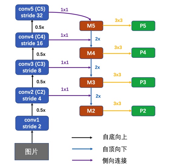
bottom up path

使用CNN进行特征提取，空间分辨率逐渐下降，语义信息逐渐增强

在bottom up path中选取的feature map是每个stage中最后一层的输出，具有该stage中最强的语义信息（输出feature map的size相同的层，统称为一个stage）

top-down pathway

对最后一层的feature map（具有最强的语义信息）进行stride=2的上采样，论文中的上采样方式为最简单的最近邻

lateral connection

横向连接为 $1×1 $ Conv，用于对 ${C_2, C_3, C_4, C_5\}$ 的channel维度进行降维（论文中设定降维后的维度为 $d = 256$ ）

注意：merged feature map 后面还需要进行 $3 \times 3$ Conv，已降低上采样带来的混叠现象（aliasing effect of upsampling）

ResNet-FPN Backbone

ResNet

使用ResNet计算多个scale的feature map
FPN

构成 feature pyramid

详见 [Feature Pyramid Network](#Feature Pyramid Network)

Classify & Regress FCN

在这里插入图片描述

Classification FCN

使用FCN，分别对Feature Pyramid的不同层的feature map进行object的classification

Output

$W \times H \times K A$ 的vector

表示每个spatial location的每个anchor都有 $K$ 个class的probability

Components

4 个 $3 \times 3$ Conv， $C$ filters（输出channel为 $C$ ）

$C$ 为输入channel数（保持channel数不变）

之后接 ReLU
1 个 $3 \times 3$ Conv， $K A$ filters（输出channel为 $K A$ ）
Sigmoid

输出每个spatial location（ $W \times H$ ）的 $A$ 个anchor的 $K$ 个类别的probability

参数共享：

subnet的参数在所有的pyramid level上共享

Regression FCN

使用FCN，分别对Feature Pyramid的不同层的feature map进行bounding box的regression

Output

$W \times H \times 4 A$ 的vector

表示每个spatial location的每个anchor都有 $4$ 个 bounding box regression

Components

除了第5层卷积输出channel为 $4 A$ ，其他与Classification FCN相同

Post Processing

对Feature Pyramid的每个level的prediction进行merge，以0.5为阈值进行NMS

两个提速技巧：

滤除confidence＜0.5的box
在每个Feature Pyramid Level上，只对1000个 top-scoring prediction进行decode

Anchor Design

scale & ratio

每个level的每个location，anchor选择3个scale，每个scale有3个ratios，共 3×3 = 9 个anchor

反应到原图上，可以覆盖32~813个pixel的范围

ratios

1: 2、1: 1、2: 1
scale

$2^0$ 、 $2^{2/3}$ 、 $2^{1/3}$

Ground Truth

每个anchor会带有2个向量

classification

一个 $K$ 维的 one-hot vector，作为classification target（ $K$ 为类别数）
regression

一个 $4$ 维的vector，作为box regression target

Anchor & GT Matching

根据anchor与ground-truth box的IOU进行匹配

IoU > 0.5

anchor被视为foreground，被分配到对应的ground-truth box

这会存在一个问题，即ground-truth box有可能对应不到anchor
0.5 > IoU > 0.4

忽略该anchor
IoU < 0.4

anchor被视为background

prior $\pi$ Initialization

在训练初期，频繁出现的类别会导致不稳定

使用 “prior” 将训练起始阶段中 rare class 的 $p$ 设定为一个较低的值（比如0.01）

用于初始化Classification SubNet的**第5个卷积层（最后一个卷积层）**的 $b$
$b=-\text{log}((1-\pi)/\pi)$

Ablation Experiments

RetinaNet $v s .$ SOTA

在这里插入图片描述

$\gamma$ on Pos & Neg Loss

在这里插入图片描述

即：Focal loss 对于foreground的loss的衰减很小 (a)，但对于background的loss衰减很大，从而避免了easy negative对于classification loss的overwhelming

AP w.r.t $\alpha_t$

在这里插入图片描述

$\alpha_t=0.5$ 对应的结果最好
$\alpha_t$ 的值也会大幅度地影响AP

AP w.r.t $\gamma$

在这里插入图片描述

$\gamma=2$ 对应的结果最好
$\gamma$ 的值也会大幅度地影响AP

FL $v s .$ OHEM

在这里插入图片描述

FL性能明显优于OHEM

AP w.r.t scale & ratio

在这里插入图片描述

scale和ratio应该兼顾
一味地堆高scale会引起效果的下降

原因可能是，这些scale本身不适合进行detection的任务

Perform w.r.t depth/scale

在这里插入图片描述

总体来说，depth和scale对performance均为正相关
- depth越深，语义信息越丰富 ==> 对small object的提升最小
- scale越大，分辨率越高，位置和细节信息越丰富 ==> 对small object的提升最大

Math

Cross Entropy Math

Standard Cross Entropy

使用 $p$ 表示
$\mathrm{CE}(p, y)=\left\{\begin{array}{ll} -\log (p) & \text { if } y=1 \\ -\log (1-p) & \text { otherwise } \end{array}\right.$
- $\in \{-1, +1\}$ ：ground-truth的class
- $\in \{ 0, 1\}$ ：预测类别为 $ 1$ 的预测概率
使用 $p_t$ 表示
$p_t=\left\{\begin{array}{ll} p& \text { if } y=1 \\ 1-p & \text { otherwise } \end{array}\right.$

$\text{CE}(p,y) = \text{CE}(p_t) = -\text{log}(p_t)$

问题：尽管每个easy sample的损失小，但大量的easy sample依旧会主导loss和gradient

Balanced Cross Entropy

$\text{CE}(p_t) = -\alpha_t \text{log}(p_t)$

$\alpha_t$ ：用于平衡正负样本

问题：仅仅是平衡正负样本，而不是难易样本，治标不治本

Focal Loss Math

$\text{FL}(p_t) = -\alpha_t·(1-p_t)^{\gamma} ·\text{log}(p_t)$

归一化系数：

匹配到ground-truth的anchor的数目
使用位置：

Classification SubNetwork ==> 仅仅是分类任务的损失函数

在这里插入图片描述

$p_t$ ：被分类正确的概率。 $p_t$ 越大，loss被down-weight的程度越大
$\gamma$ ：控制down-weight的程度
- 实验中 $\gamma=2$ 最好
- $\gamma=0$ 时，FL Loss = CE Loss

求导：
$\frac{d\text{FL}}{d x}=y\left(1-p_{t}\right)^{\gamma}\left(\gamma p_{t} \log \left(p_{t}\right)+p_{t}-1\right)$

Use Yourself

Data Analysis

数据分析能力是至关重要的：“做机器学习首先要是数据科学家”

面对一项任务，了解其数据的分布是至关重要的一环，这会建立起你对该任务面对的状况（尤其是困难）的直观的认识

良好的数据分布会给后续的操作带来良好的基础，在一些方面也具有优良的性质

Focal Loss就是数据分布上起作用的

[Feature Pyramid Network](#Feature Pyramid Network)

Feature Pyramid Network 其实是一种将语义信息和细节/位置信息结合的方式，处理了feature map结合时的size不符的问题，可以较好的结合不同scale的feature map的优点

Feature Pyramid Network 提取到的特征兼顾了多种分辨率和强语义信息，可以广泛地用于后续的处理（特征工程？）

Feature Pyramid Network 从更广义上来讲，其实是给出了一种信息聚合的结构，可以结合带有不同属性的同种信息

More Scale $\not= $ Better

详见 [Perform w.r.t depth/scale](#Perform w.r.t depth/scale)

一味地增加feature map的multi-scale并不是总能带来性能的提升

feature map的level的选取，也需要合理去选择

并不是拉过来一个feature map就能用！！！

Related Work

Two-Stage Method

Characteristic

精度高，速度慢

Input

分类器的输入为稀疏的候选目标集（sparse set of candidate object locations）

Sampling Fashion

stage-1 ==> proposal stage

生成稀疏的候选目标集（sparse set of candidate object locations）

滤除绝大部分的 background samples
stage-2 ==> classification stage

使用分类器进行分类，最终结果为 foreground classes / background

在这阶段会采用 sampling heuristics，老保持foreground和background的平衡
- fixed foreground-to-background ratio (1: 3)
- Hard Negative Mining ==> Online Hard Example Mining