


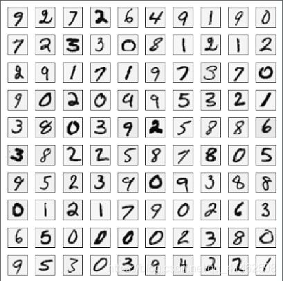
数据可视化
还是像前一个联系一样,首先进行数据可视化:
import matplotlib.pyplot as plt
import numpy as np
import scipy.io as sio
import matplotlib
import scipy.optimize as opt
from sklearn.metrics import classification_report#这个包是评价报告
def load_data(path,transpose=True):
    data=sio.loadmat(path)
    y=data.get("y")
    y=y.reshape(y.shape[0])
    X=data.get("X")
    if transpose:
        X=np.array([im.reshape(20,20).T for im in X])
        X=np.array([im.reshape(400) for im in X])
    return X,y
X,_=load_data("code/ex4-NN back propagation/ex4data1.mat")#在这里我们暂时不用y所以先丢弃
def plot_100_image(X):
    size=int(np.sqrt(X.shape[1]))
    sample_idx=np.random.choice(np.arange(X.shape[0]),100)
    sample_img=X[sample_idx,:]
    fig,ax_array=plt.subplots(ncols=10,nrows=10,sharex=True,sharey=True,figsize=(8,8))
    for r in range(10):
        for c in range(10):
            ax_array[r,c].matshow(sample_img[10*r+c].reshape(size,size), cmap=matplotlib.cm.binary)
            plt.xticks(np.array([]))
            plt.yticks(np.array([]))
plot_100_image(X)
plt.show()
读取权重
def load_weight(path):
    data = sio.loadmat(path)
    return data['Theta1'], data['Theta2']
t1,t2=load_weight("code/ex4-NN back propagation/ex4weights.mat")
print(t1.shape)
print(t2.shape)
(25, 401)
(10, 26)
def serialize(a,b):
    return np.concatenate((np.ravel(a),np.ravel(b)))
theta=serialize(t1,t2)#25*401+10*26
theta.shape
(10285,)
def deserialize(seq):
    t1=seq[:25*401].reshape(25,401)
    t2=seq[25*401:].reshape(10,26)
    return t1,t2
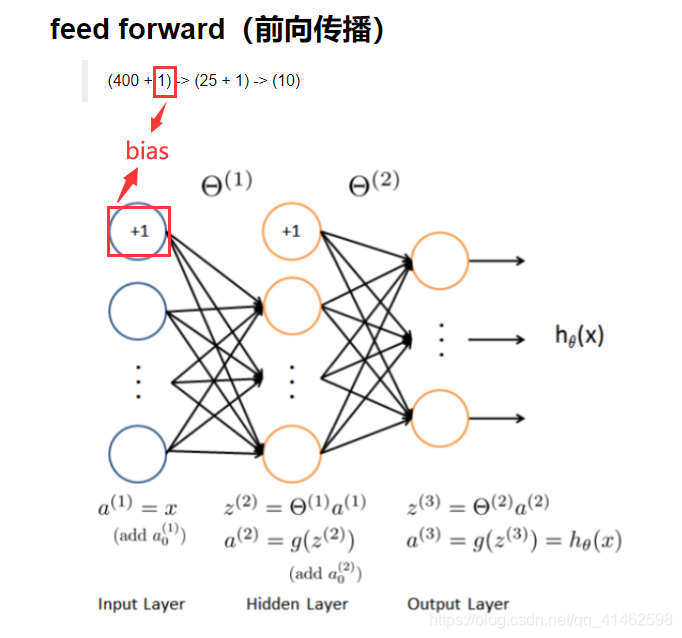
前向传播
X_raw, y_raw = load_data('code/ex4-NN back propagation/ex4data1.mat', transpose=False)
X = np.insert(X_raw, 0, np.ones(X_raw.shape[0]), axis=1)#增加全部为1的一列
X.shape
(5000, 401)
对y标签进行一次one-hot 编码。 one-hot 编码将类标签n(k类)转换为长度为k的向量,其中索引n为“hot”(1),而其余为0。 Scikitlearn有一个内置的实用程序,我们可以使用这个。
from sklearn.preprocessing import OneHotEncoder
encoder = OneHotEncoder(sparse=False)
y = encoder.fit_transform(y_raw)
y.shape
(5000, 10)
def feed_forward(theta,X):
    t1,t2=deserialize(theta)#t1(25,401),t2(10,26)
    m=X.shape[0]#5000个样本
    a1=X#第一层输入(5000,401)
    z2=a1@t1.T #(5000,401)@(401,25)=(5000,25)
    a2=sigmoid(z2)#(5000,25)
    a2=np.insert(a2,0,np.ones(m),axis=1)#5000*26
    z3=a2@t2.T#(5000,26)@(26,10)=(5000,10)
    h=sigmoid(z3)#5000*10
    return a1,z2,a2,z3,h#反向传播中会用到
def sigmoid(z):
    return 1/(1+np.exp(-z))
_,_,_,_,h=feed_forward(theta,X)
h
array([[1.12661530e-04, 1.74127856e-03, 2.52696959e-03, …,
4.01468105e-04, 6.48072305e-03, 9.95734012e-01],
[4.79026796e-04, 2.41495958e-03, 3.44755685e-03, …,
2.39107046e-03, 1.97025086e-03, 9.95696931e-01],
[8.85702310e-05, 3.24266731e-03, 2.55419797e-02, …,
6.22892325e-02, 5.49803551e-03, 9.28008397e-01],
…,
[5.17641791e-02, 3.81715020e-03, 2.96297510e-02, …,
2.15667361e-03, 6.49826950e-01, 2.42384687e-05],
[8.30631310e-04, 6.22003774e-04, 3.14518512e-04, …,
1.19366192e-02, 9.71410499e-01, 2.06173648e-04],
[4.81465717e-05, 4.58821829e-04, 2.15146201e-05, …,
5.73434571e-03, 6.96288990e-01, 8.18576980e-02]
代价函数
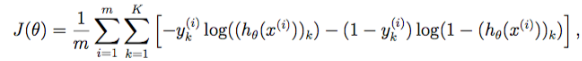
k是总共的类别数量,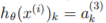
表示第k个输出单元
def cost(theta,X,y):
    m=X.shape[0]
    _,_,_,_,h=feed_forward(theta,X)
    inner=-y*np.log(h)-(1-y)*np.log(1-h)
    cost=np.sum(inner)/m
    return cost
cost(theta,X,y)
0.2876291651613189
正则化代价函数
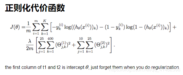
def regularized_cost(theta,X,y,l=1):
    t1,t2=deserialize(theta)
    m=X.shape[0]
    reg_t1=(1/(2*m))*np.sum(np.power(t1[:,1:],2))
    reg_t2=(1/(2*m))*np.sum(np.power(t2[:,1:],2))
    return cost(theta,X,y)+reg_t1+reg_t2
regularized_cost(theta,X,y)
0.38376985909092365
反向传播
def sigmoid_gradient(z):
    return np.multiply(sigmoid(z),1-sigmoid(z))
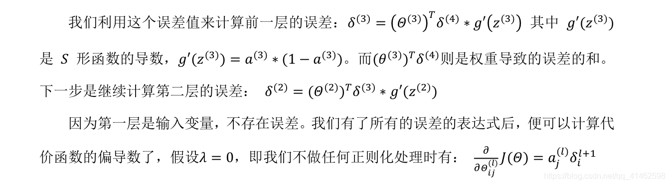
def gradient(theta,X,y):
    t1,t2=deserialize(theta)#t1: (25,401) t2: (10,26)
    m=X.shape[0]
    delta1=np.zeros(t1.shape)#(25,401)
    delta2=np.zeros(t2.shape)#(10,26)
    a1,z2,a2,z3,h=feed_forward(theta,X)
    # (5000,401),(5000,25),(5000,26),(5000,10),(5000,10)
    for i in range(m):
        a1i=a1[i,:]#(401,)
        z2i=z2[i,:]#(25,)
        a2i=a2[i,:]#(26,1)
        z3i=z3[i,:]#(10,)
        hi=h[i,:]#(10,)
        yi=y[i,:]#(10,)
        d3i=hi-yi#(10,)
        z2i=np.insert(z2i,0,np.ones(1))#因为要通过a2i来计算梯度,a2i是(26,),所以说反向传播时让z2i变为(26,)来计算d2i
        d2i=np.multiply(t2.T@d3i,sigmoid_gradient(z2i))
        #有了上一层的误差过后,便可以计算代价函数的偏导数了
        delta2+=np.matrix(d3i).T@np.matrix(a2i)#(10,1)@(1,26)
        delta1+=np.matrix(d2i[1:]).T@np.matrix(a1i)#算误差的时候不用算之前加上的bias 所以从位置1开始,维度为(1,25).T@(1,401)
    delta1 = delta1 / m
    delta2 = delta2 / m
    # print(z2i.shape) (26,)
    # print(np.matrix(z2i).shape) (1,26)
    return serialize(delta1, delta2)
d1, d2 = deserialize(gradient(theta, X, y))
d1.shape, d2.shape
((25, 401), (10, 26))
正则化梯度下降
def regularized_gradient(theta,X,y,l=1):
    m=X.shape[0]
    delta1,delta2=deserialize(gradient(theta,X,y))
    t1,t2=deserialize(theta)#t1: (25,401) t2: (10,26)
    t1[:,0]=0#x0不惩罚
    reg_term_d1=(l/m)*t1
    delta1=delta1+reg_term_d1
    t2[:,0]=0#x0不惩罚
    reg_term_d2=(l/m)*t2
    delta2=delta2+reg_term_d2
    return serialize(delta1,delta2)
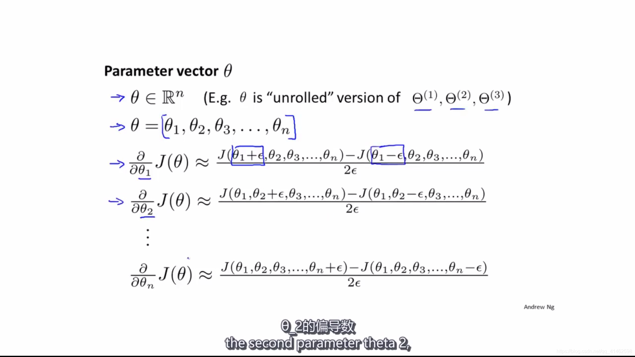
梯度校验
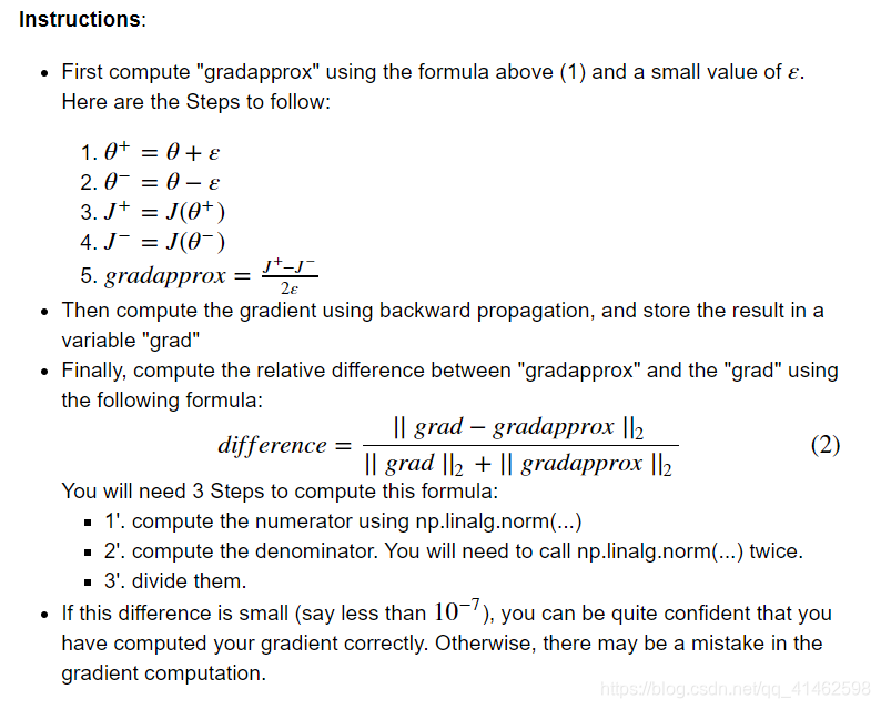
当θ是一个向量时,我们则需要对偏导数进行检验,因为代价函数的偏导数只针对一个参数的改变进行检验,下面是检验的示例
def expand_array(arr):
    """replicate array into matrix
    [1, 2, 3]

    [[1, 2, 3],
     [1, 2, 3],
     [1, 2, 3]]
    """
    # turn matrix back to ndarray
    return np.array(np.matrix(np.ones(arr.shape[0])).T @ np.matrix(arr))
def gradient_checking(theta, X, y, epsilon, regularized=False):

    theta_matrix = expand_array(theta)  # expand to (10285, 10285)
    epsilon_matrix = np.identity(len(theta)) * epsilon#(10285,10285)的单位矩阵
    #因为代价函数的偏导数只针对一个参数的改变进行检验
    plus_matrix = theta_matrix + epsilon_matrix
    minus_matrix = theta_matrix - epsilon_matrix
    def a_numeric_grad(plus, minus, regularized=False):
        """calculate a partial gradient with respect to 1 theta"""
        if regularized:
            return (regularized_cost(plus, X, y) - regularized_cost(minus, X, y)) / (epsilon * 2)
        else:
            return (cost(plus, X, y) - cost(minus, X, y)) / (epsilon * 2)

    # calculate numerical gradient with respect to all theta
    numeric_grad = np.array([a_numeric_grad(plus_matrix[i], minus_matrix[i], regularized)
                                    for i in range(len(theta))])

    # analytical grad will depend on if you want it to be regularized or not
    analytic_grad = regularized_gradient(theta, X, y) if regularized else gradient(theta, X, y)

    # If you have a correct implementation, and assuming you used EPSILON = 0.0001
    # the diff below should be less than 1e-9
    # this is how original matlab code do gradient checking
    diff = np.linalg.norm(numeric_grad - analytic_grad) / np.linalg.norm(numeric_grad + analytic_grad)

    print('If your backpropagation implementation is correct,\nthe relative difference will be smaller than 10e-9 (assume epsilon=0.0001).\nRelative Difference: {}\n'.format(diff))
gradient_checking(theta, X, y, epsilon= 0.0001)
If your backpropagation implementation is correct,
the relative difference will be smaller than 10e-9 (assume epsilon=0.0001).
Relative Difference: 2.1457557907925204e-09
开始训练模型
1.随机初始化
def random_init(size):
    return np.random.uniform(-0.12,0.12,size)
def nn_training(X,y):
    init_theta=random_init(10285)
    res=opt.minimize(fun=regularized_cost,x0=init_theta,args=(X,y,1),method="TNC",jac=regularized_gradient,options={'maxiter': 400})
    return res
res = nn_training(X, y)#慢
res
fun: 0.3296362256102031
jac: array([ 1.12252251e-04, -1.04461635e-06, -6.21429981e-07, …,
-1.39037086e-04, -6.24049316e-05, 2.57115389e-08])
message: ‘Linear search failed’
nfev: 386
nit: 22
status: 4
success: False
x: array([ 0. , -0.00522308, -0.00310715, …, 1.62836521,
1.70377569, -0.0211097 ])
_, y_answer = load_data('code/ex4-NN back propagation/ex4data1.mat')
final_theta = res.x
def show_accuracy(theta, X, y):
    _, _, _, _, h = feed_forward(theta, X)

    y_pred = np.argmax(h, axis=1) + 1

    print(classification_report(y, y_pred))
show_accuracy(final_theta,X,y_answer)
precision recall f1-score support
      1       0.99      0.98      0.99       500
      2       0.84      1.00      0.91       500
      3       0.92      0.98      0.95       500
      4       0.98      0.97      0.98       500
      5       1.00      0.74      0.85       500
      6       0.99      0.98      0.98       500
      7       1.00      0.89      0.94       500
      8       0.94      0.99      0.96       500
      9       0.96      0.98      0.97       500
     10       0.92      1.00      0.96       500
avg / total 0.95 0.95 0.95 5000


 285
285

 被折叠的 条评论
为什么被折叠?
被折叠的 条评论
为什么被折叠?
 到【灌水乐园】发言


