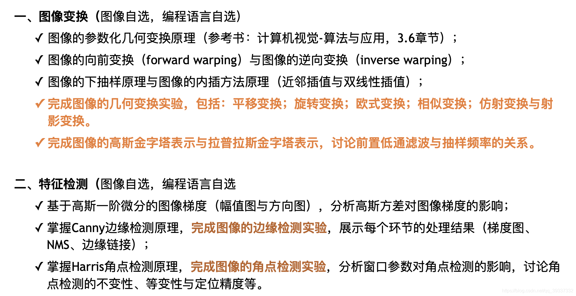
Inverse Geometric Transform； Gaussian and Laplacian Pyramid； Canny Filter； Harris Detection从零实现

这是本学期选修的Computer Vision and Pattern Recognition的第一次作业，主要要求是

import numpy as np
from math import floor, cos, sin, pi, exp
from PIL import Image
import matplotlib.pyplot as plt
from pprint import pprint
%matplotlib inline

image_lenna = Image.open('lenna.jpg')
image_lenna = image_lenna.resize((480, 480))
image_lenna = image_lenna.convert('L')  
image_lenna = np.asarray(image_lenna)

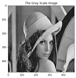
plt.figure(figsize=(5, 5))
plt.imshow(image_lenna, cmap=plt.cm.gray)
plt.title('The Gray Scale Image')

Geometric Transform

To implement inverse warp, the first thing is to implement interpolate function. Here I just use bilinear method.

Interpolate function

def interpolate(image, subpixel, method="bilinear"):
    if method == "bilinear":
        pixel = [floor(p) for p in subpixel]
        delta = [sub - p for sub, p in zip(subpixel, pixel)]
        surroundings = np.array([image[pixel[0], pixel[1]],
                                 image[pixel[0] + 1, pixel[1]],
                                 image[pixel[0], pixel[1] + 1],
                                 image[pixel[0] + 1, pixel[1] + 1]])
        weight = np.array([(1 - delta[0]) * (1 - delta[1]),
                           delta[0] * (1 - delta[1]),
                           (1 - delta[0]) * delta[1],
                           delta[0] * delta[1]])
        inter = np.sum(weight * surroundings)
        return int(inter)

Consider the homogenous point of a 2D geometric plane:
$$\mathbf{p}=[xy1{]}^T$$Define a transform function:
$$T\in {\mathbb{R}}^{3\times 3}$$Then the homogenous point after transform is
$${\mathbf{p}}_{\mathrm{n}\mathrm{e}\mathrm{w}}=T\mathbf{p}$$where ${\mathbf{p}}_{\mathrm{n}\mathrm{e}\mathrm{w}}=\frac{{\mathbf{p}}_{\mathrm{n}\mathrm{e}\mathrm{w}}}{{\mathbf{p}}_{\mathrm{n}\mathrm{e}\mathrm{w}}^z}$ under homogenous coordinate system. So first I implement the most basic transform function.

Transform function

def transform(image, T):
    image_pad = np.pad(image, ((0,1), (0,1)), 'edge')
    src_shape = image.shape
    T_inv = np.linalg.inv(T)
    # calculate image range
    canvas = np.array([[0, src_shape[1], 1], 
                      [src_shape[0], 0, 1], 
                      [src_shape[0], src_shape[1], 1], 
                      [0, 0, 1]])
    canvas = np.transpose(canvas)
    T_canvas = np.trunc(np.matmul(T, canvas))
    T_canvas[0, :] = np.true_divide(T_canvas[0, :], T_canvas[2, :])
    T_canvas[1, :] = np.true_divide(T_canvas[1, :], T_canvas[2, :])
    
    mins = np.min(T_canvas, axis=1)
    maxs = np.max(T_canvas, axis=1)
    dst_range = [[int(mins[0]), int(maxs[0])], [int(mins[1]), int(maxs[1])]]
    dst_image = 255 * np.ones([dst_range[0][1] - dst_range[0][0], 
                               dst_range[1][1] - dst_range[1][0]])
    
    for x in range(dst_range[0][0], dst_range[0][1]):
        for y in range(dst_range[1][0], dst_range[1][1]):
            T_xy = np.array([x, y])
            T_xy1 = np.array([x, y, 1])
            xy1 = np.matmul(T_inv, T_xy1)
            
            xy1[0] = xy1[0] / xy1[2]
            xy1[1] = xy1[1] / xy1[2]
            
            xy = xy1[:2]
            mat_xy = [T_xy[0]-dst_range[0][0], T_xy[1]-dst_range[1][0]]
            if (0 <= xy[0] < src_shape[0]-1) and (0 <= xy[1] < src_shape[1]-1):
                dst_image[mat_xy[0], mat_xy[1]] = np.array(interpolate(image_pad, xy))
            else:
                dst_image[mat_xy[0], mat_xy[1]] = np.array([255])
    return dst_image, dst_range

Define a plot function to visulize the result.

plot function

def plot(image, ranges, scale=1, title=""):
    plt.figure(figsize=(scale*5, scale*5))
    plt.imshow(image/255, cmap=plt.cm.gray)
    plt.title(title)
    plt.xticks(range(0, image.shape[1], 100), labels=range(ranges[1][0], ranges[1][1], 100))
    plt.yticks(range(0, image.shape[0], 100), labels=range(ranges[0][0], ranges[0][1], 100))

Transforms

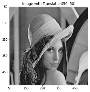
Translation

Translation means that
$$T=\left[\begin{array}{ccc}1& 0& T_x\\ 0& 1& T_y\\ 0& 0& 1\end{array}\right]$$

def translation(image, shift):
    T = np.array([[1, 0, shift[0]], 
                  [0, 1, shift[1]], 
                  [0, 0, 1]])
    return transform(image, T)

i, r = translation(image_lenna, [50, 50])
plot(i, r, title="Image with Translation(50, 50)")

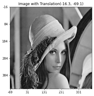
i, r = translation(image_lenna, [-16.3, -69.1])
plot(i, r, title="Image with Translation(-16.3, -69.1)")

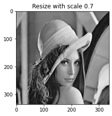
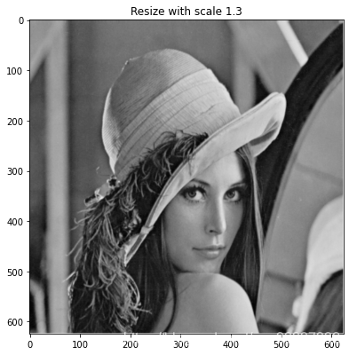
Resize

Resize means that
$$T=\left[\begin{array}{ccc}s& 0& 0\\ 0& s& 0\\ 0& 0& 1\end{array}\right]$$

def resize(image, scale):
    T = np.array([[scale, 0, 0], 
                  [0, scale, 0], 
                  [0, 0, 1]])
    return transform(image, T)

i, r = resize(image_lenna, 0.7)
plot(i, r, title="Resize with scale 0.7", scale=0.7)

i, r = resize(image_lenna, 1.3)
plot(i, r, title="Resize with scale 1.3", scale=1.3)

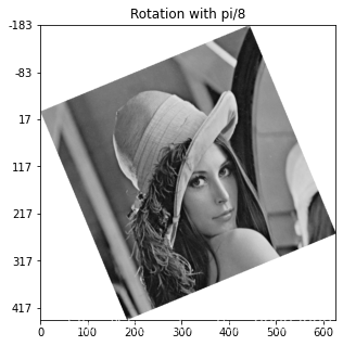
Rotation

Rotation means that
$$T=\left[\begin{array}{ccc}\cos (\theta )& -\sin (\theta )& 0\\ \sin (\theta )& \cos (\theta )& 0\\ 0& 0& 1\end{array}\right]$$

def rotation(image, theta):
    T = np.array([[cos(theta), -sin(theta), 0], 
                  [sin(theta), cos(theta), 0], 
                  [0, 0, 1]])
    return transform(image, T)

i, r = rotation(image_lenna, pi/8)
plot(i, r, title="Rotation with pi/8")

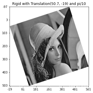
Rigid

Rigid means that
$$T=\left[\begin{array}{ccc}\cos (\theta )& -\sin (\theta )& T_x\\ \sin (\theta )& \cos (\theta )& T_y\\ 0& 0& 1\end{array}\right]$$

def rigid(image, shift, theta):
    T = np.array([[cos(theta), -sin(theta), shift[0]], 
                  [sin(theta), cos(theta), shift[1]], 
                  [0, 0, 1]])
    return transform(image, T)

i, r = rigid(image_lenna, [50.7, -19], pi/10)
plot(i, r, title="Rigid with Translation(50.7, -19) and pi/10")

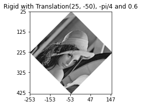
Similarity

Rigid means that
$$T=\left[\begin{array}{ccc}s\cos (\theta )& -s\sin (\theta )& T_x\\ s\sin (\theta )& s\cos (\theta )& T_y\\ 0& 0& 1\end{array}\right]$$

def similarity(image, shift, theta, scale):
    T = np.array([[scale * cos(theta), -scale * sin(theta), shift[0]], 
                  [scale * sin(theta), scale * cos(theta), shift[1]], 
                  [0, 0, 1]])
    return transform(image, T)

i, r = similarity(image_lenna, [25, -50], -pi/4, 0.6)
plot(i, r, title="Rigid with Translation(25, -50), -pi/4 and 0.6", scale=0.6)

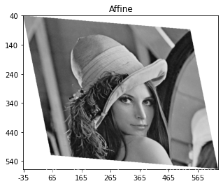
Affine

Affine means that
$$T=\left[\begin{array}{ccc}a& b& T_x\\ c& d& T_y\\ 0& 0& 1\end{array}\right]$$

def affine(image, A, shift):
    T = np.array([[A[0][0], A[0][1], shift[0]], 
                  [A[1][0], A[1][1], shift[1]], 
                  [0, 0, 1]])
    return transform(image, T)

i, r = affine(image_lenna, A=[[1, 0.1], [0.2, 1.2]], shift=[40, -35.4])
plot(i, r, title="Affine")

Projection

Projection means that
$$T=\left[\begin{array}{ccc}a& b& T_x\\ c& d& T_y\\ e& f& 1\end{array}\right]$$

def project(image, A, shift, v):
    T = np.array([[A[0][0], A[0][1], shift[0]], 
                  [A[1][0], A[1][1], shift[1]], 
                  [v[0], v[1], 1]])
    return transform(image, T)

i, r = project(image_lenna, A=[[1, 0.1], [0.2, 1.2]], shift=[70, -35.4], v=[0.001, 0.002])
plot(i, r, title="Projection")

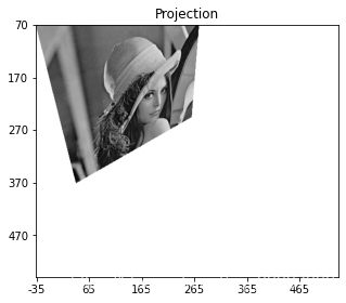
Image Pyramid

Convolution

First define the gaussian filter with kernel size equals to 5, notice that it is a estimation of original 2D gaussian distribution samples.

Gaussia_kernel = (1/256) * np.array([[1, 4, 6, 4, 1], 
                                     [4, 16, 24, 16, 4], 
                                     [6, 24, 36, 24, 6], 
                                     [4, 16, 24, 16, 4], 
                                     [1, 4, 6, 4, 1]])

Define the convolution operation with the image padded by half of the kernel size.

def conv(image, kernel):
    kernel_size = kernel.shape[0]
#     image_pad = np.zeros([image.shape[0]+4, image.shape[1]+4])
#     kernels = np.zeros([kernel_size, kernel_size])
    
    image_pad = np.pad(image, ((2,2), (2,2)), 'edge')
#     kernels[:, :] = kernel
        
    dst_image = np.zeros([image.shape[0], image.shape[1]])
    dst_shape = dst_image.shape
    for x in range(dst_shape[0]):
        for y in range(dst_shape[1]):
            surroudings = image_pad[x:x+kernel_size, y:y+kernel_size]
            conv_rslt = surroudings * kernel
            dst_image[x, y] = np.sum(np.sum(conv_rslt, axis=0), axis=0)
            
    return dst_image

downSample

Gaussian down sample operation. First convolute it with gaussian kernel and then take out the odd rows and columns.

def GauDown(image, kernel, step=2):
    image_conv = conv(image, kernel)
    image_down = image_conv[::step, ::step]
    return image_down

upSample

Gaussian down sample operation. First interplote it with rows and columns of zeros and then filte it with gaussian kernel.

def GauUp(image, kernel, step=2):
    src_shape = image.shape
    image_up = np.zeros([src_shape[0]*2, src_shape[1]*2])
    for x in range(src_shape[0]):
        for y in range(src_shape[1]):
            image_up[2*x+1, 2*y+1] = image[x, y]
    image_conv = conv(image_up, kernel)
    image_up[::2, ::2] = image_conv[::step, ::step]
    return image_conv

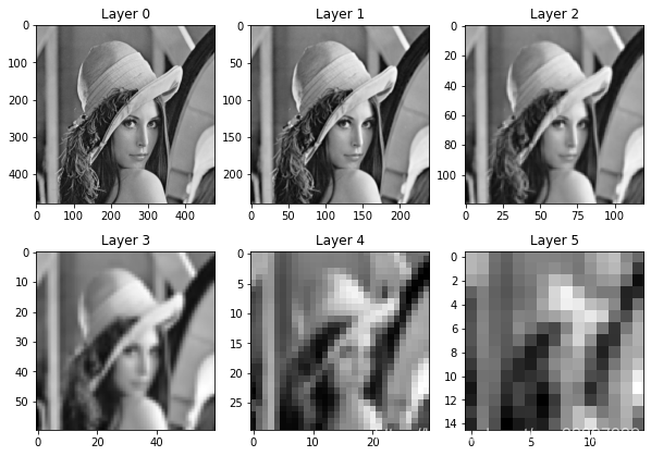
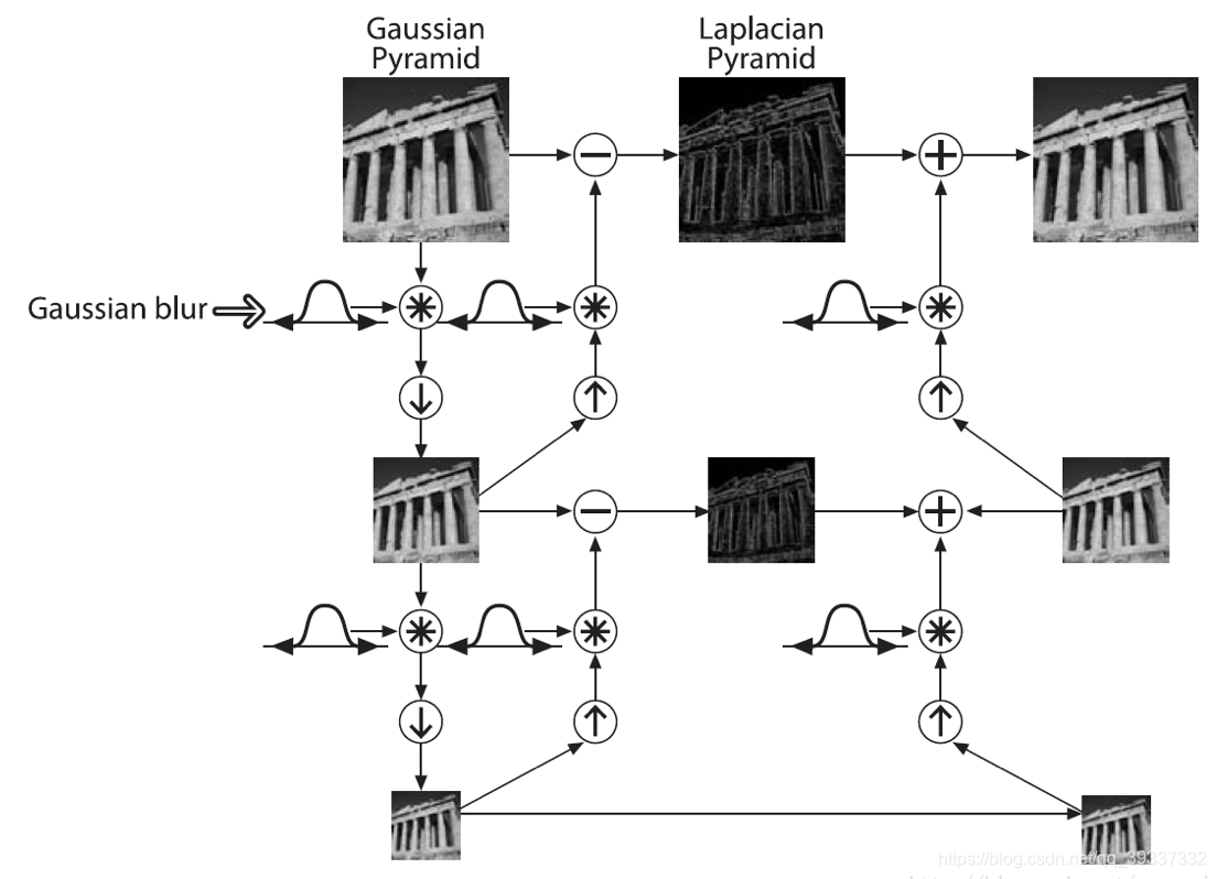
Gaussian Pyramid

Built the Gaussian Pyramid.

GauPry = [image_lenna]
num_layer = 5
img = image_lenna
for _ in range(num_layer):
    image_down = GauDown(img, Gaussia_kernel)
    GauPry.append(image_down)
    img = image_down

plt.figure(figsize=(10, 7))
for i in range(len(GauPry)):
    plt.subplot(2, 3, i+1)
    plt.imshow(GauPry[i]/255., cmap=plt.cm.gray)
    plt.title('Layer ' + str(i))

Now consider the new image is generated by sample the image of step 2, 3, 4, 5 seperately:

GauPry_step = [image_lenna]
steps = [2, 3, 4, 5]
for step in steps:
    image_down = GauDown(image_lenna, Gaussia_kernel, step)
    GauPry_step.append(image_down)

plt.figure(figsize=(25, 25))
plt.subplot(1, 5, 1)
plt.imshow(GauPry_step[0]/255., cmap=plt.cm.gray)
plt.title('Original image')
for i in range(len(steps)):
    plt.subplot(1, 5, i+2)
    plt.imshow(GauPry_step[i+1]/255., cmap=plt.cm.gray)
    plt.title('step ' + str(steps[i]))

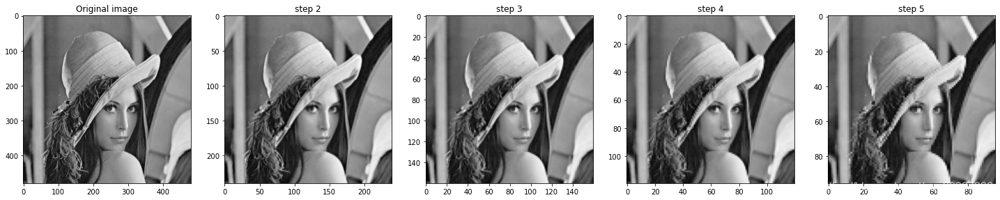
As we can observe, the images of different downsample do not vary a lot. The pre filter ensure that image can be robust to sample rate.

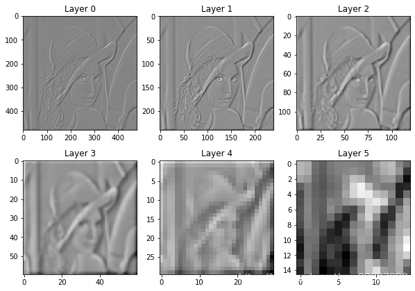
Laplacian Pyramid

The calculation of Laplacian Pyramid is
$$L_i=G_i-PyrUp(G_{i+1})$$
which is shown as below

GauExpand = []
for i in range(num_layer):
    image_up = GauUp(GauPry[i+1], 4*Gaussia_kernel)
    GauExpand.append(image_up)

LapPry = []
for i in range(num_layer):
    LapPry.append(GauPry[i] - GauExpand[i])
LapPry.append(GauPry[-1])

plt.figure(figsize=(10, 7))
for i in range(len(LapPry)):
    plt.subplot(2, 3, i+1)
    if i == 5:
        plt.imshow(LapPry[i]/255., cmap=plt.cm.gray)
    else:
        plt.imshow(LapPry[i], cmap=plt.cm.gray)
    plt.title('Layer ' + str(i))

Feature Detection

Gaussian derivative

filter kernels

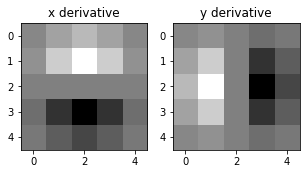
First we define the derivative of 2d gaussian distribution along x and y according to
$$\begin{array}{r}\frac{\partial G}{\partial x}=-\frac{x}{{\sigma }^2}G\\ \frac{\partial G}{\partial y}=-\frac{y}{{\sigma }^2}G\end{array}$$

def gaussian_dx(sigma, x, y):
    gaussian_xy = 1/(2*pi*sigma**2) * exp(-(x**2+y**2)/(2*sigma**2))
    return -x/sigma**2 * gaussian_xy

def gaussian_dy(sigma, x, y):
    gaussian_xy = 1/(2*pi*sigma**2) * exp(-(x**2+y**2)/(2*sigma**2))
    return -y/sigma**2 * gaussian_xy

def get_gaussian_kernel(sigma, kernel_size, direction):
    Gaussian_d_kernel = np.zeros([kernel_size, kernel_size])
    for x in range(kernel_size):
        for y in range(kernel_size):
            if direction == 'x':
                Gaussian_d_kernel[x, y] = gaussian_dx(sigma, x-kernel_size//2, y-kernel_size//2)
            elif direction == 'y':
                Gaussian_d_kernel[x, y] = gaussian_dy(sigma, x-kernel_size//2, y-kernel_size//2)
    return Gaussian_d_kernel

Gaussian_dx_kernel = get_gaussian_kernel(1, 5, 'x')
Gaussian_dy_kernel = get_gaussian_kernel(1, 5, 'y')

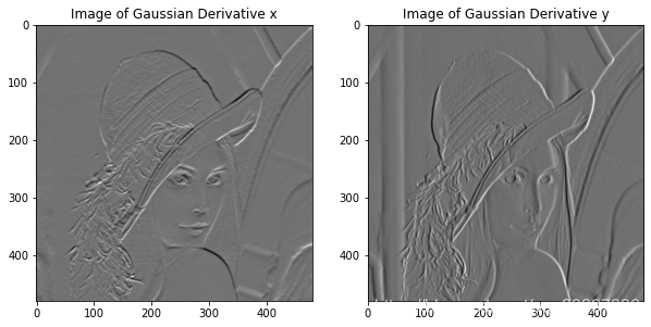
Here is the plots of 2 partial gaussian distribution with window size equals to 5.

plt.figure(figsize=(5, 5))
plt.subplot(121)
plt.imshow(Gaussian_dx_kernel, cmap=plt.cm.gray)
plt.title('x derivative')
plt.subplot(122)
plt.imshow(Gaussian_dy_kernel, cmap=plt.cm.gray)
plt.title('y derivative')

magnitude and direction

image_gaussian_dx = conv(image_lenna, Gaussian_dx_kernel)
image_gaussian_dy = conv(image_lenna, Gaussian_dy_kernel)

plt.figure(figsize=(10, 10))
plt.subplot(121)
plt.imshow(image_gaussian_dx/image_gaussian_dx.max(), cmap=plt.cm.gray)
plt.title('Image of Gaussian Derivative x')
plt.subplot(122)
plt.imshow(image_gaussian_dy/image_gaussian_dy.max(), cmap=plt.cm.gray)
plt.title('Image of Gaussian Derivative y')

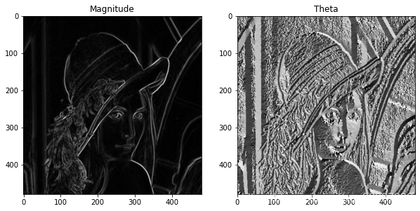
To accelerate calculation, I use the $|I_x|+|I_y|$ to estimate magnitude. And the direction is calculated by $\arctan \frac{I_y}{I_x}$.

def get_gaussian_derivative(image, sigma):
    _dx_kernel = get_gaussian_kernel(sigma, 5, 'x')
    _dy_kernel = get_gaussian_kernel(sigma, 5, 'y')
    _image_dx = conv(image, _dx_kernel)
    _image_dy = conv(image, _dy_kernel)
    mag = np.abs(_image_dx) + np.abs(_image_dy)
    theta = np.arctan2(_image_dy, _image_dx)
    
    return mag, theta

mag, theta = get_gaussian_derivative(image_lenna, 1)

plt.figure(figsize=(10, 10))
plt.subplot(121)
plt.imshow(mag/mag.max(), cmap=plt.cm.gray)
plt.title('Magnitude')
plt.subplot(122)
plt.imshow(theta/theta.max(), cmap=plt.cm.gray)
plt.title('Theta')

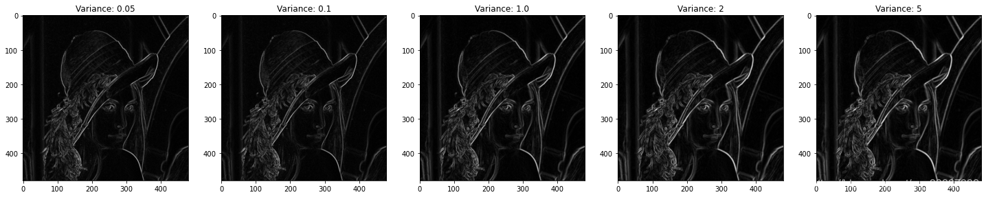
The influence of Gaussian variance

mags = []
thetas = []
sigmas = [0.05, 1e-1, 1e0, 2, 5]
for i in range(len(sigmas)):
    mag, theta = get_gaussian_derivative(image_lenna, sigmas[i])
    mags.append(mag)
    thetas.append(theta)

plt.figure(figsize=(25, 25))
for i in range(5):
    mag = mags[i]
    plt.subplot(1, 5, i+1)
    plt.imshow(mag/mag.max(), cmap=plt.cm.gray)
    plt.title("Variance: " + str(sigmas[i]))

plt.figure(figsize=(25, 25))
for i in range(5):
    theta = thetas[i]
    plt.subplot(1, 5, i+1)
    plt.imshow(theta/theta.max(), cmap=plt.cm.gray)
    plt.title("Variance: " + str(sigmas[i]))

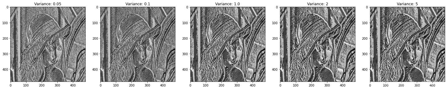
We can see that as var gets bigger, more details of the image are revealed.

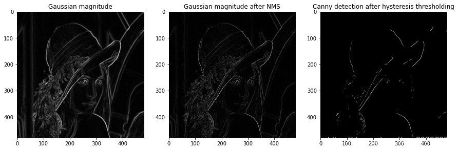
Canny filter

I implement canny filter according to the following 4 steps:
1) Filter image with x, y derivatives of Gaussian
2) Find magnitude and orientation of gradient
3) Non maximum surppress
4) Hysteresis thresholding

Filter image with x, y derivatives of Gaussian

dx_kernel = get_gaussian_kernel(1, 5, 'x')
dy_kernel = get_gaussian_kernel(1, 5, 'y')
image_dx = conv(image_lenna, dx_kernel)
image_dy = conv(image_lenna, dy_kernel)

Find magnitude and orientation of gradient

mag, theta = get_gaussian_derivative(image_lenna, 1)

NMS

The pricinpal of nms is stated as followed:
1) take the direction $g$ at point $q=(x,y)$
2) calculate $r=q+\frac{g}{||g||}$ and $p=q-\frac{g}{||g||}$
3) compare the magtitude at $q,r,p$ (maybe sub-pixel) if magtitude of $p$ is max, then save it as maximum.

def interpolate_single(image, subpixel, method="bilinear"):
    if method == "bilinear":
        pixel = [floor(p) for p in subpixel]
        delta = [sub - p for sub, p in zip(subpixel, pixel)]
        surroundings = np.array([image[pixel[0], pixel[1]],
                                 image[pixel[0] + 1, pixel[1]],
                                 image[pixel[0], pixel[1] + 1],
                                 image[pixel[0] + 1, pixel[1] + 1]]).reshape([4, 1])
        weight = np.array([(1 - delta[0]) * (1 - delta[1]),
                           delta[0] * (1 - delta[1]),
                           (1 - delta[0]) * delta[1],
                           delta[0] * delta[1]]).reshape([4, 1])
        
        inter = np.sum(weight * surroundings, axis=0)
        return inter

def nms(image_dx, image_dy, mag):
    image_shape = image_dx.shape
#     image_nms = np.zeros([image_shape[0], image_shape[1]])
    
    dx_pad = np.pad(image_dx, ((1, 1), (1, 1)), 'edge')
    dy_pad = np.pad(image_dy, ((1, 1), (1, 1)), 'edge')
    mag_pad = np.pad(mag, ((1, 1), (1, 1)), 'edge')

    for x in range(1, image_shape[0]+1):
        for y in range(1, image_shape[1]+1):
            q = np.array([x, y])
            g = np.array([dx_pad[x, y], dy_pad[x, y]])

            r = q + g/np.linalg.norm(g)
            mag_r = interpolate_single(mag_pad, r)
            p = q - g/np.linalg.norm(g)
            mag_p = interpolate_single(mag_pad, p)
            if (mag_pad[x, y] > mag_p[0]) and (mag_pad[x, y] > mag_r[0]):
                pass
            else:
                mag_pad[x, y] = 0

    image_nms = mag_pad[1:image_shape[0]+1, 1:image_shape[1]+1]
    return image_nms

image_nms = nms(image_dx, image_dy, mag)

hysteresis threshold

Here I use a mask to represent the position of high pixel value and medium pixel value to calculate.

def hysteresis(image, low, high):
    image_shape = image.shape
#     image_hyster = np.zeros([image_shape[0], image_shape[1]])
    
    image_single = image / image.max()
    boundary = np.zeros([image_shape[0], image_shape[1]])

    image_high_mask = image_single >= high
    image_middle_mask = image_single >= low

    for x in range(1, image_shape[0]-1):
        for y in range(1, image_shape[1]-1):
            if image_high_mask[x, y] == True:
                boundary[x-1:x+1, y-1:y+1] = image_single[x-1:x+1, y-1:y+1] * image_middle_mask[x-1:x+1, y-1:y+1]
    
    image_hyster = boundary
    
    return image_hyster

image_hyster = hysteresis(image_nms, 0.1, 0.5)

plt.figure(figsize=(15, 15))
plt.subplot(131)
plt.imshow(mag/mag.max(), cmap=plt.cm.gray)
plt.title("Gaussian magnitude")
plt.subplot(132)
plt.imshow(image_nms/image_nms.max(), cmap=plt.cm.gray)
plt.title("Gaussian magnitude after NMS")
plt.subplot(133)
plt.imshow(image_hyster/image_hyster.max(), cmap=plt.cm.gray)
plt.title("Canny detection after hysteresis thresholding")

Harris detection

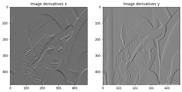
I implement harris detection of its Harris88 version:
1) Image derivatives
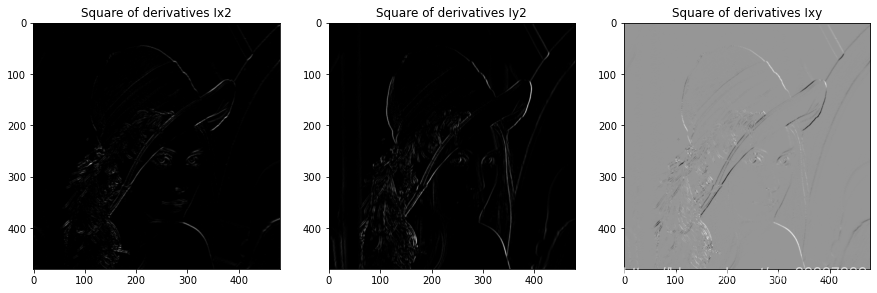
2) Square of derivatives
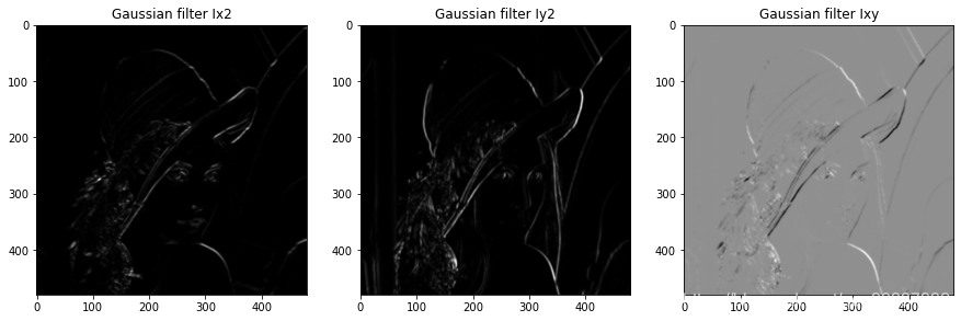
3) Gaussian filter
4) Calculate cornerness function $har=g(I_x^2)g(I_y^2)-g(I_x{I}_y{)}^2-\alpha [g(I_x^2)+g(I_y^2){]}^2$
5) NMS

def harris(image, window_size=5, alpha=0.05):
    image_shape = image.shape
    
    sobel_x = np.array([[1, 2, 1], [0, 0, 0], [-1, -2, -1]])
    sobel_y = np.array([[-1, 0, 1], [-2, 0, 2], [-1, 0, 1]])
    window = 1.0 * np.ones([window_size, window_size])
    dst_image = np.ones([image_shape[0], image_shape[1]])
    R = np.ones([image_shape[0], image_shape[1]])
    
    Ix = conv(image, sobel_x)
    Iy = conv(image, sobel_y)
    
    Ix2 = Ix * Ix
    Iy2 = Iy * Iy
    Ixy = Ix * Iy

    Gaussia_kernel = (1/256) * np.array([[1, 4, 6, 4, 1], 
                                         [4, 16, 24, 16, 4], 
                                         [6, 24, 36, 24, 6], 
                                         [4, 16, 24, 16, 4], 
                                         [1, 4, 6, 4, 1]])
    gIx2 = conv(Ix2, Gaussia_kernel)
    gIy2 = conv(Iy2, Gaussia_kernel)
    gIxy = conv(Ixy, Gaussia_kernel)
    har = gIx2*gIy2 - gIxy*gIxy - alpha*(gIx2+gIy2)*(gIx2+gIy2)
    har = conv(har, Gaussia_kernel)
    return har, Ix, Iy, Ix2, Iy2, Ixy, gIx2, gIy2, gIxy

har, Ix, Iy, Ix2, Iy2, Ixy, gIx2, gIy2, gIxy = harris(image_lenna)

Image derivatives

plt.figure(figsize=(10, 10))
plt.subplot(121)
plt.imshow(Ix/Ix.max(), cmap=plt.cm.gray)
plt.title('Image derivatives x')
plt.subplot(122)
plt.imshow(Iy/Iy.max(), cmap=plt.cm.gray)
plt.title('Image derivatives y')

Square of derivatives

plt.figure(figsize=(15, 15))
plt.subplot(131)
plt.imshow(Ix2/Ix2.max(), cmap=plt.cm.gray)
plt.title('Square of derivatives Ix2')
plt.subplot(132)
plt.imshow(Iy2/Iy2.max(), cmap=plt.cm.gray)
plt.title('Square of derivatives Iy2')
plt.subplot(133)
plt.imshow(Ixy/Ixy.max(), cmap=plt.cm.gray)
plt.title('Square of derivatives Ixy')

Gaussian filter

plt.figure(figsize=(15, 15))
plt.subplot(131)
plt.imshow(gIx2/gIx2.max(), cmap=plt.cm.gray)
plt.title('Gaussian filter Ix2')
plt.subplot(132)
plt.imshow(gIy2/gIy2.max(), cmap=plt.cm.gray)
plt.title('Gaussian filter Iy2')
plt.subplot(133)
plt.imshow(gIxy/gIxy.max(), cmap=plt.cm.gray)
plt.title('Gaussian filter Ixy')

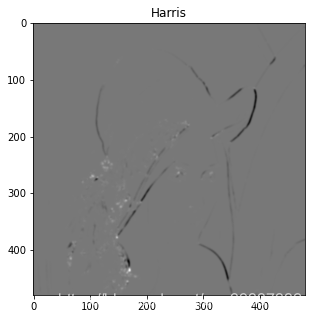
cornerness function

plt.figure(figsize=(5, 5))
plt.imshow((har-har.min())/(har.max()-har.min()), cmap=plt.cm.gray)
plt.title('Harris')

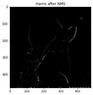
NMS

# NMS as the last step of harris detection
mag, theta = get_gaussian_derivative(har, 1)
dx_kernel = get_gaussian_kernel(1, 5, 'x')
dy_kernel = get_gaussian_kernel(1, 5, 'y')
image_dx = conv(har, dx_kernel)
image_dy = conv(har, dy_kernel)
image_nms = nms(image_dx, image_dy, mag)

plt.figure(figsize=(5, 5))
plt.imshow(image_nms/image_nms.max(), cmap=plt.cm.gray)
plt.title('Harris after NMS')

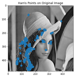
har_norm = (har-har.min())/(har.max()-har.min())
points = np.where(har_norm >= np.percentile(har_norm, 99))
plt.figure(figsize=(5, 5))
plt.imshow(image_lenna, cmap=plt.cm.gray)
plt.scatter(points[1], points[0])
plt.title('Harris Points on Original Image')

alphas = [0.01, 0.02, 0.05, 0.1, 1]
hars = []
for alpha in alphas:
    output = harris(image_lenna, alpha=alpha)
    har = output[0]
    har = (har - har.min()) / (har.max() - har.min())
    hars.append(har)

plt.figure(figsize=(25, 25))
for i in range(len(alphas)):
    har_norm = hars[i]
    points = np.where(har_norm >= np.percentile(har_norm, 99))
    plt.subplot(1, len(alphas), i+1)
    plt.imshow(image_lenna, cmap=plt.cm.gray)
    plt.scatter(points[1], points[0])
    plt.title('Harris with alpha=' + str(alphas[i]))

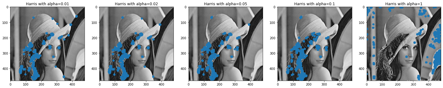
I adjust the hyper-parameter $\alpha$, we can see that as it get bigger, the harris detection result gets more blur.

Transform invariance

lenna_affine, r = affine(image_lenna, A=[[1, 0.1], [0.2, 1.2]], shift=[40, -35.4])
output = harris(lenna_affine, alpha=0.05)
har = output[0]
har_norm = (har-har.min()) / (har.max()-har.min())
points = np.where(har_norm >= np.percentile(har_norm, 99))

plt.figure(figsize=(5, 5))
plt.imshow(lenna_affine/lenna_affine.max(), cmap=plt.cm.gray)
plt.xticks(range(0, lenna_affine.shape[1], 100), labels=range(r[1][0], r[1][1], 100))
plt.yticks(range(0, lenna_affine.shape[0], 100), labels=range(r[0][0], r[0][1], 100))
plt.scatter(points[1], points[0])
plt.title('Harris Points on Affine Image')

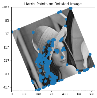
lenna_rotation, r = rotation(image_lenna, pi/8)
output = harris(lenna_rotation, alpha=0.05)
har = output[0]
har_norm = (har-har.min()) / (har.max()-har.min())
points = np.where(har_norm >= np.percentile(har_norm, 99))
plt.figure(figsize=(5, 5))
plt.imshow(lenna_rotation/lenna_rotation.max(), cmap=plt.cm.gray)
plt.xticks(range(0, lenna_rotation.shape[1], 100), labels=range(r[1][0], r[1][1], 100))
plt.yticks(range(0, lenna_rotation.shape[0], 100), labels=range(r[0][0], r[0][1], 100))
plt.scatter(points[1], points[0])
plt.title('Harris Points on Rotated Image')

lenna_scale, r = resize(image_lenna, 0.7)
output = harris(lenna_scale, alpha=0.05)
har = output[0]
har_norm = (har-har.min()) / (har.max()-har.min())
points = np.where(har_norm >= np.percentile(har_norm, 99))
plt.figure(figsize=(5, 5))
plt.imshow(lenna_scale/lenna_scale.max(), cmap=plt.cm.gray)
plt.xticks(range(0, lenna_scale.shape[1], 100), labels=range(r[1][0], r[1][1], 100))
plt.yticks(range(0, lenna_scale.shape[0], 100), labels=range(r[0][0], r[0][1], 100))
plt.scatter(points[1], points[0])
plt.title('Harris Points on Scaled Image')

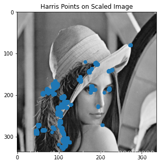
As the image is affined, the harris detection do not change a lot. We can oberseve that harris detection is invariant to affine, rotation and scale.