大市场销售预测项目_机器学习案例实战零售商品销售预测big mart使用最少三种不同的算法-优快云博客

本文链接：https://blog.youkuaiyun.com/qq_39297053/article/details/137204991

该项目旨在分析BigMart销售数据，预测产品在特定商店的销售额。处理流程包括数据预处理、探索性数据分析、特征选择等。选用线性回归、决策树等模型，经评估优化后分析结果并提出业务改进建议。项目面临高维数据、模型泛化等挑战。

摘要生成于 C知道，由 DeepSeek-R1 满血版支持，前往体验 >

注意：本文引用自专业人工智能社区Venus AI

项目概述

这个项目的主要目标是分析BigMart的销售数据，从而预测不同产品在特定商店的销售额。通过这种方式，可以揭示影响销售的关键因素，并为商店的库存管理、定价策略和市场营销活动提供数据支持。项目的处理流程如下：

数据集特征描述

Item_Identifier：物品标识符。
Item_Weight：产品的重量。
Item_Fat_Content：产品的脂肪含量（低脂、常规等）。
Item_Visibility：产品在商店中的可见度。
Item_Type：物品种类。
Item_MRP：最大零售价（MRP）。
Outlet_Identifier：商店的唯一ID。
Outlet_Establishment_Year：商店成立的年份。
Outlet_Size：商店的大小。
Outlet_Location_Type：商店的位置类型（城市、郊区等）。
Outlet_Type：商店的类型（如超市、杂货店）。
Item_Outlet_Sales：产品在特定商店的销售额（目标变量）。

数据预处理

缺失值处理：分析并填补或删除缺失的数据。
数据清洗：处理不一致的分类数据和异常值。
特征工程：创建新特征或转换现有特征以提高模型性能。

探索性数据分析（EDA）

统计分析：使用描述性统计分析数据的中心趋势和分布。
可视化：绘制条形图、箱形图、散点图等，以了解各变量间的关系。

特征选择

确定对销售额预测最重要的特征。
可能需要进行特征编码（如独热编码）以适应模型。

模型与依赖

选择模型：根据问题的性质选择合适的预测模型，如线性回归、决策树、随机森林等。
训练模型：使用训练数据集训练模型。

本项目的科学计算库依赖：

matplotlib==3.7.1
numpy==1.24.3
pandas==2.0.2
plotly==5.18.0
scikit_learn==1.2.2
seaborn==0.13.0

模型评估与优化

使用测试集评估模型的准确性。
通过交叉验证、调整超参数等方法来优化模型。

结果解释与应用

分析并解释模型结果，理解影响销售额的主要因素。
提出基于数据的业务改进建议，如库存优化、定价策略调整。

项目挑战

高维数据：需要有效的特征选择和降维技术。
模型的泛化能力：确保模型在未知数据上的表现。
数据质量：数据的准确性和完整性对最终结果至关重要。

项目的代码详情：

# Importing the libraries
import numpy as np
import pandas as pd
import matplotlib.pyplot as plt
import seaborn as sns
import plotly.express as px
from sklearn.preprocessing import LabelEncoder
from sklearn.model_selection import train_test_split
from sklearn.linear_model import LinearRegression
%matplotlib inline

train = pd.read_csv('Train.csv')
test = pd.read_csv('Test.csv')

train.shape,test.shape

((8523, 12), (5681, 11))

查询空值

train.isnull().sum()

Item_Identifier                 0
Item_Weight                  1463
Item_Fat_Content                0
Item_Visibility                 0
Item_Type                       0
Item_MRP                        0
Outlet_Identifier               0
Outlet_Establishment_Year       0
Outlet_Size                  2410
Outlet_Location_Type            0
Outlet_Type                     0
Item_Outlet_Sales               0
dtype: int64

test.isnull().sum()

Item_Identifier                 0
Item_Weight                   976
Item_Fat_Content                0
Item_Visibility                 0
Item_Type                       0
Item_MRP                        0
Outlet_Identifier               0
Outlet_Establishment_Year       0
Outlet_Size                  1606
Outlet_Location_Type            0
Outlet_Type                     0
dtype: int64

train.isnull().sum()/train.shape[0]*100 == train.isnull().sum()/train.shape[0]*100

Item_Identifier              True
Item_Weight                  True
Item_Fat_Content             True
Item_Visibility              True
Item_Type                    True
Item_MRP                     True
Outlet_Identifier            True
Outlet_Establishment_Year    True
Outlet_Size                  True
Outlet_Location_Type         True
Outlet_Type                  True
Item_Outlet_Sales            True
dtype: bool

train.info()

<class 'pandas.core.frame.DataFrame'>
RangeIndex: 8523 entries, 0 to 8522
Data columns (total 12 columns):
 #   Column                     Non-Null Count  Dtype  
---  ------                     --------------  -----  
 0   Item_Identifier            8523 non-null   object 
 1   Item_Weight                7060 non-null   float64
 2   Item_Fat_Content           8523 non-null   object 
 3   Item_Visibility            8523 non-null   float64
 4   Item_Type                  8523 non-null   object 
 5   Item_MRP                   8523 non-null   float64
 6   Outlet_Identifier          8523 non-null   object 
 7   Outlet_Establishment_Year  8523 non-null   int64  
 8   Outlet_Size                6113 non-null   object 
 9   Outlet_Location_Type       8523 non-null   object 
 10  Outlet_Type                8523 non-null   object 
 11  Item_Outlet_Sales          8523 non-null   float64
dtypes: float64(4), int64(1), object(7)
memory usage: 799.2+ KB

train.describe()

	Item_Weight	Item_Visibility	Item_MRP	Outlet_Establishment_Year	Item_Outlet_Sales
count	7060.000000	8523.000000	8523.000000	8523.000000	8523.000000
mean	12.857645	0.066132	140.992782	1997.831867	2181.288914
std	4.643456	0.051598	62.275067	8.371760	1706.499616
min	4.555000	0.000000	31.290000	1985.000000	33.290000
25%	8.773750	0.026989	93.826500	1987.000000	834.247400
50%	12.600000	0.053931	143.012800	1999.000000	1794.331000
75%	16.850000	0.094585	185.643700	2004.000000	3101.296400
max	21.350000	0.328391	266.888400	2009.000000	13086.964800

test.info()

<class 'pandas.core.frame.DataFrame'>
RangeIndex: 5681 entries, 0 to 5680
Data columns (total 11 columns):
 #   Column                     Non-Null Count  Dtype  
---  ------                     --------------  -----  
 0   Item_Identifier            5681 non-null   object 
 1   Item_Weight                4705 non-null   float64
 2   Item_Fat_Content           5681 non-null   object 
 3   Item_Visibility            5681 non-null   float64
 4   Item_Type                  5681 non-null   object 
 5   Item_MRP                   5681 non-null   float64
 6   Outlet_Identifier          5681 non-null   object 
 7   Outlet_Establishment_Year  5681 non-null   int64  
 8   Outlet_Size                4075 non-null   object 
 9   Outlet_Location_Type       5681 non-null   object 
 10  Outlet_Type                5681 non-null   object 
dtypes: float64(3), int64(1), object(7)
memory usage: 488.3+ KB

test.describe()

	Item_Weight	Item_Visibility	Item_MRP	Outlet_Establishment_Year
count	4705.000000	5681.000000	5681.000000	5681.000000
mean	12.695633	0.065684	141.023273	1997.828903
std	4.664849	0.051252	61.809091	8.372256
min	4.555000	0.000000	31.990000	1985.000000
25%	8.645000	0.027047	94.412000	1987.000000
50%	12.500000	0.054154	141.415400	1999.000000
75%	16.700000	0.093463	186.026600	2004.000000
max	21.350000	0.323637	266.588400	2009.000000

train.columns

Index(['Item_Identifier', 'Item_Weight', 'Item_Fat_Content', 'Item_Visibility',
       'Item_Type', 'Item_MRP', 'Outlet_Identifier',
       'Outlet_Establishment_Year', 'Outlet_Size', 'Outlet_Location_Type',
       'Outlet_Type', 'Item_Outlet_Sales'],
      dtype='object')

检查数据中的异常值

fig = px.box(train,y = 'Item_Weight')
fig.show()

fig = px.box(test,y = 'Item_Weight')
fig.show()

由于数据中不存在异常值，因此我们通过存在的其他值的平均值来估算 Item_Weight 中的空值。

train['Item_Weight'] = train['Item_Weight'].fillna(train['Item_Weight'].mean())
test['Item_Weight'] = test['Item_Weight'].fillna(test['Item_Weight'].mean())

train.isnull().sum()

Item_Identifier                 0
Item_Weight                     0
Item_Fat_Content                0
Item_Visibility                 0
Item_Type                       0
Item_MRP                        0
Outlet_Identifier               0
Outlet_Establishment_Year       0
Outlet_Size                  2410
Outlet_Location_Type            0
Outlet_Type                     0
Item_Outlet_Sales               0
dtype: int64

test.isnull().sum()

Item_Identifier                 0
Item_Weight                     0
Item_Fat_Content                0
Item_Visibility                 0
Item_Type                       0
Item_MRP                        0
Outlet_Identifier               0
Outlet_Establishment_Year       0
Outlet_Size                  1606
Outlet_Location_Type            0
Outlet_Type                     0
dtype: int64

train['Outlet_Size'].value_counts()

Medium    2793
Small     2388
High       932
Name: Outlet_Size, dtype: int64

test['Outlet_Size'].value_counts()

Medium    1862
Small     1592
High       621
Name: Outlet_Size, dtype: int64

通过将其替换为众数（即最常出现的值）来删除空值。

train['Outlet_Size'] = train['Outlet_Size'].fillna(train['Outlet_Size'].mode()[0])
test['Outlet_Size'] = test['Outlet_Size'].fillna(test['Outlet_Size'].mode()[0])

train.isnull().sum()

Item_Identifier              0
Item_Weight                  0
Item_Fat_Content             0
Item_Visibility              0
Item_Type                    0
Item_MRP                     0
Outlet_Identifier            0
Outlet_Establishment_Year    0
Outlet_Size                  0
Outlet_Location_Type         0
Outlet_Type                  0
Item_Outlet_Sales            0
dtype: int64

test.isnull().sum()

Item_Identifier              0
Item_Weight                  0
Item_Fat_Content             0
Item_Visibility              0
Item_Type                    0
Item_MRP                     0
Outlet_Identifier            0
Outlet_Establishment_Year    0
Outlet_Size                  0
Outlet_Location_Type         0
Outlet_Type                  0
dtype: int64

train.head()

	Item_Identifier	Item_Weight	Item_Fat_Content	Item_Visibility	Item_Type	Item_MRP	Outlet_Identifier	Outlet_Establishment_Year	Outlet_Size	Outlet_Location_Type	Outlet_Type	Item_Outlet_Sales
0	FDA15	9.30	Low Fat	0.016047	Dairy	249.8092	OUT049	1999	Medium	Tier 1	Supermarket Type1	3735.1380
1	DRC01	5.92	Regular	0.019278	Soft Drinks	48.2692	OUT018	2009	Medium	Tier 3	Supermarket Type2	443.4228
2	FDN15	17.50	Low Fat	0.016760	Meat	141.6180	OUT049	1999	Medium	Tier 1	Supermarket Type1	2097.2700
3	FDX07	19.20	Regular	0.000000	Fruits and Vegetables	182.0950	OUT010	1998	Medium	Tier 3	Grocery Store	732.3800
4	NCD19	8.93	Low Fat	0.000000	Household	53.8614	OUT013	1987	High	Tier 3	Supermarket Type1	994.7052

train['Item_Fat_Content'].value_counts()

Low Fat    5089
Regular    2889
LF          316
reg         117
low fat     112
Name: Item_Fat_Content, dtype: int64

删除数据集中的名词定义不规则之处。

train['Item_Fat_Content'].replace(['low fat','LF','reg'],['Low Fat','Low Fat','Regular'],inplace = True)

train['Item_Fat_Content'].value_counts()

Low Fat    5517
Regular    3006
Name: Item_Fat_Content, dtype: int64

test.head()

	Item_Identifier	Item_Weight	Item_Fat_Content	Item_Visibility	Item_Type	Item_MRP	Outlet_Identifier	Outlet_Establishment_Year	Outlet_Size	Outlet_Location_Type	Outlet_Type
0	FDW58	20.750000	Low Fat	0.007565	Snack Foods	107.8622	OUT049	1999	Medium	Tier 1	Supermarket Type1
1	FDW14	8.300000	reg	0.038428	Dairy	87.3198	OUT017	2007	Medium	Tier 2	Supermarket Type1
2	NCN55	14.600000	Low Fat	0.099575	Others	241.7538	OUT010	1998	Medium	Tier 3	Grocery Store
3	FDQ58	7.315000	Low Fat	0.015388	Snack Foods	155.0340	OUT017	2007	Medium	Tier 2	Supermarket Type1
4	FDY38	12.695633	Regular	0.118599	Dairy	234.2300	OUT027	1985	Medium	Tier 3	Supermarket Type3

test['Item_Fat_Content'].value_counts()

Low Fat    3396
Regular    1935
LF          206
reg          78
low fat      66
Name: Item_Fat_Content, dtype: int64

test['Item_Fat_Content'].replace(['low fat','LF','reg'],['Low Fat','Low Fat','Regular'],inplace = True)

test['Item_Fat_Content'].replace(['low fat','LF','reg'],['Low Fat','Low Fat','Regular'],inplace = True)

Low Fat    3668
Regular    2013
Name: Item_Fat_Content, dtype: int64

train['Years in Bussiness'] = train['Outlet_Establishment_Year'].apply(lambda x:2022-x)
test['Years in Bussiness'] = test['Outlet_Establishment_Year'].apply(lambda x:2022-x)

train.head()

	Item_Identifier	Item_Weight	Item_Fat_Content	Item_Visibility	Item_Type	Item_MRP	Outlet_Identifier	Outlet_Establishment_Year	Outlet_Size	Outlet_Location_Type	Outlet_Type	Item_Outlet_Sales	Years in Bussiness
0	FDA15	9.30	Low Fat	0.016047	Dairy	249.8092	OUT049	1999	Medium	Tier 1	Supermarket Type1	3735.1380	23
1	DRC01	5.92	Regular	0.019278	Soft Drinks	48.2692	OUT018	2009	Medium	Tier 3	Supermarket Type2	443.4228	13
2	FDN15	17.50	Low Fat	0.016760	Meat	141.6180	OUT049	1999	Medium	Tier 1	Supermarket Type1	2097.2700	23
3	FDX07	19.20	Regular	0.000000	Fruits and Vegetables	182.0950	OUT010	1998	Medium	Tier 3	Grocery Store	732.3800	24
4	NCD19	8.93	Low Fat	0.000000	Household	53.8614	OUT013	1987	High	Tier 3	Supermarket Type1	994.7052	35

fig = px.histogram(train,x = 'Item_Fat_Content')
fig.show()

fig = px.histogram(train,x = 'Item_Type')
fig.show()

fig = px.histogram(train,'Outlet_Size')
fig.show()

fig = px.histogram(train,'Outlet_Location_Type')
fig.show()

fig = px.histogram(train,'Outlet_Type')
fig.show()

fig = px.histogram(train,'Years in Bussiness')
fig.show()

fig = px.scatter(train,x = 'Item_MRP',y = 'Item_Outlet_Sales')
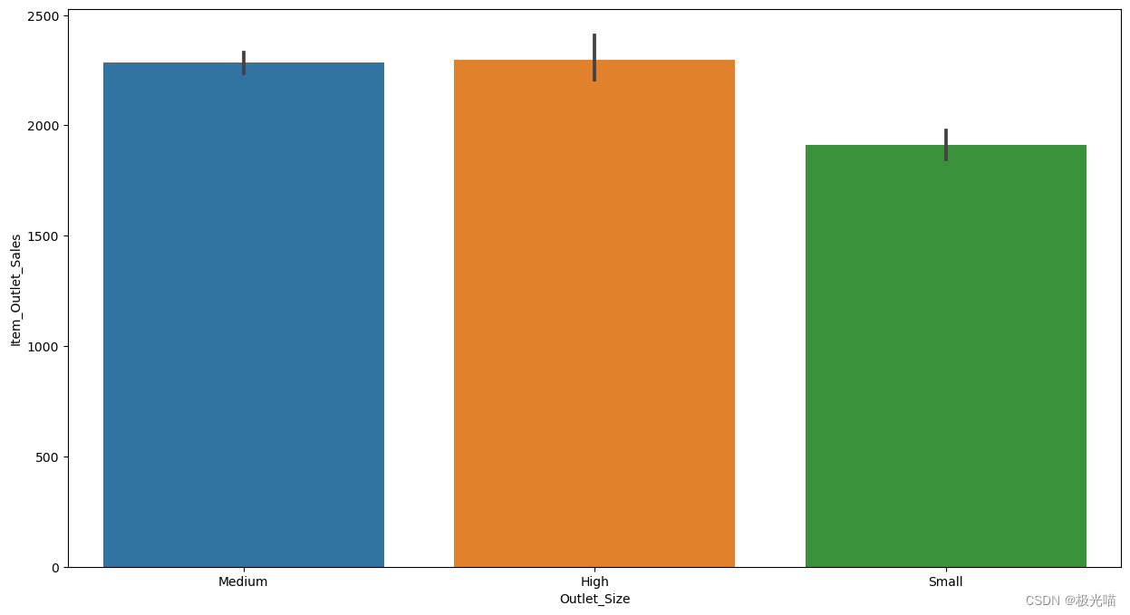
fig.show()

plt.figure(figsize = (15,8))
sns.barplot(data = train,x = 'Outlet_Size',y = 'Item_Outlet_Sales')

<Axes: xlabel='Outlet_Size', ylabel='Item_Outlet_Sales'>

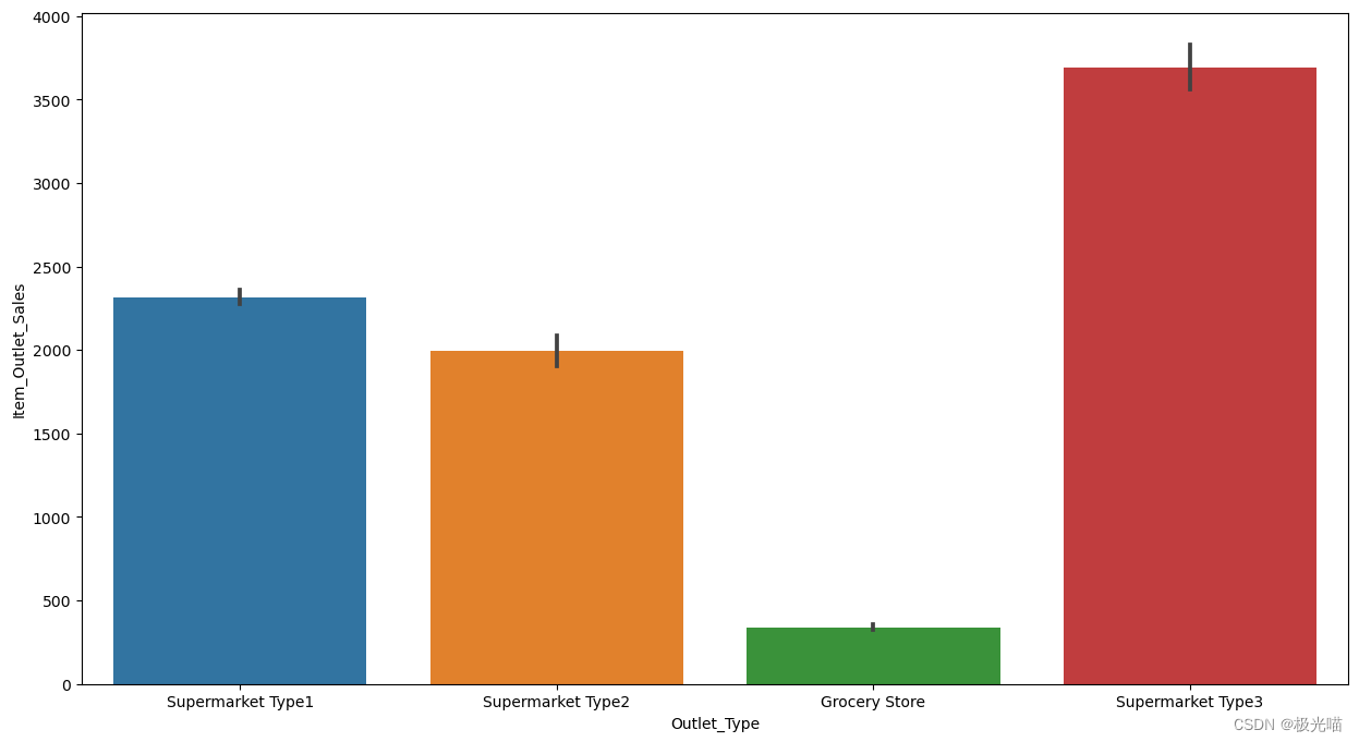
plt.figure(figsize = (15,8))
sns.barplot(data = train,x = 'Outlet_Type',y = 'Item_Outlet_Sales')

<Axes: xlabel='Outlet_Type', ylabel='Item_Outlet_Sales'>

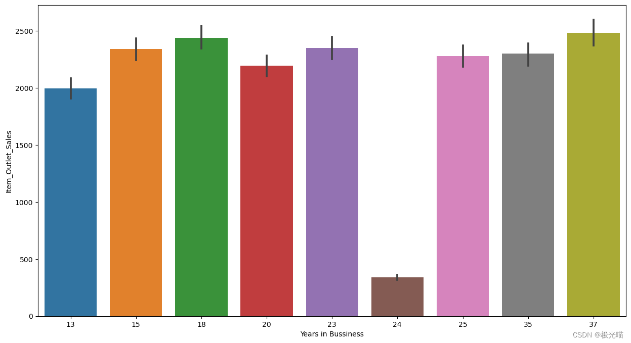
plt.figure(figsize = (15,8))
sns.barplot(data = train,x = 'Years in Bussiness',y = 'Item_Outlet_Sales')

<Axes: xlabel='Years in Bussiness', ylabel='Item_Outlet_Sales'>

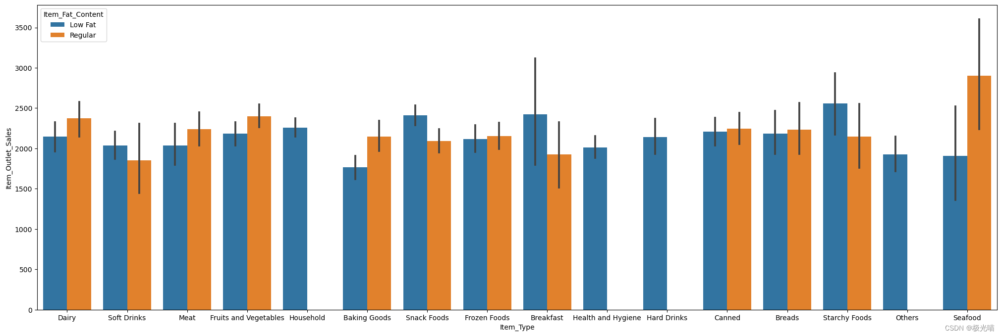
plt.figure(figsize = (25,8))
sns.barplot(x = 'Item_Type',y = 'Item_Outlet_Sales',hue = 'Item_Fat_Content',data = train)

<Axes: xlabel='Item_Type', ylabel='Item_Outlet_Sales'>

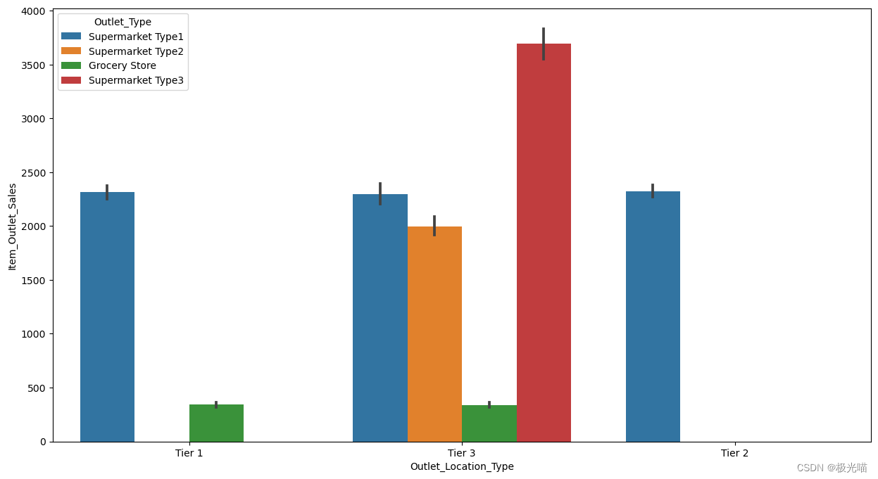
plt.figure(figsize = (15,8))
sns.barplot(x = 'Outlet_Location_Type',y = 'Item_Outlet_Sales',data = train,hue = 'Outlet_Type')

<Axes: xlabel='Outlet_Location_Type', ylabel='Item_Outlet_Sales'>

train.head()

	Item_Identifier	Item_Weight	Item_Fat_Content	Item_Visibility	Item_Type	Item_MRP	Outlet_Identifier	Outlet_Establishment_Year	Outlet_Size	Outlet_Location_Type	Outlet_Type	Item_Outlet_Sales	Years in Bussiness
0	FDA15	9.30	Low Fat	0.016047	Dairy	249.8092	OUT049	1999	Medium	Tier 1	Supermarket Type1	3735.1380	23
1	DRC01	5.92	Regular	0.019278	Soft Drinks	48.2692	OUT018	2009	Medium	Tier 3	Supermarket Type2	443.4228	13
2	FDN15	17.50	Low Fat	0.016760	Meat	141.6180	OUT049	1999	Medium	Tier 1	Supermarket Type1	2097.2700	23
3	FDX07	19.20	Regular	0.000000	Fruits and Vegetables	182.0950	OUT010	1998	Medium	Tier 3	Grocery Store	732.3800	24
4	NCD19	8.93	Low Fat	0.000000	Household	53.8614	OUT013	1987	High	Tier 3	Supermarket Type1	994.7052	35

le = LabelEncoder()
categorical = ['Item_Fat_Content','Item_Type','Outlet_Size','Outlet_Location_Type','Outlet_Type']
for ele in categorical:
    train[ele] = le.fit_transform(train[ele])
for ele in categorical:
    test[ele] = le.fit_transform(test[ele])

train.columns

Index(['Item_Identifier', 'Item_Weight', 'Item_Fat_Content', 'Item_Visibility',
       'Item_Type', 'Item_MRP', 'Outlet_Identifier',
       'Outlet_Establishment_Year', 'Outlet_Size', 'Outlet_Location_Type',
       'Outlet_Type', 'Item_Outlet_Sales', 'Years in Bussiness'],
      dtype='object')

test.columns

Index(['Item_Identifier', 'Item_Weight', 'Item_Fat_Content', 'Item_Visibility',
       'Item_Type', 'Item_MRP', 'Outlet_Identifier',
       'Outlet_Establishment_Year', 'Outlet_Size', 'Outlet_Location_Type',
       'Outlet_Type', 'Years in Bussiness'],
      dtype='object')

X = train[['Item_Weight', 'Item_Fat_Content', 'Item_Visibility',
       'Item_Type', 'Item_MRP', 'Outlet_Size', 'Outlet_Location_Type',
       'Outlet_Type', 'Years in Bussiness']]
y = train['Item_Outlet_Sales']

X_train,X_test,y_train,y_test = train_test_split(X,y,test_size = 0.33,random_state=101)

lr = LinearRegression()

lr.fit(X_train,y_train)

LinearRegression

LinearRegression()

predictions = lr.predict(X_test)

from sklearn.metrics import r2_score,mean_absolute_error

r2_score(y_test,predictions)

0.5181645537014002

mean_absolute_error(y_test,predictions)

861.5671749460174

from sklearn.ensemble import RandomForestRegressor

rf = RandomForestRegressor(n_estimators=200,max_depth = 5,min_samples_leaf = 100,n_jobs = 4,random_state = 101)
rf.fit(X_train,y_train)
pred = rf.predict(X_test)

print(mean_absolute_error(y_test,pred))
print(r2_score(y_test,pred))

731.7911976837737
0.6060286599205379

因此，显然，随机森林回归器表现更好

项目资源下载

详情请见大市场销售预测项目-VenusAI (aideeplearning.cn)

结论

这个项目涉及到数据预处理、探索性分析、特征工程、模型选择和优化等多个方面，是一个综合性的数据科学项目。通过这个项目，可以获得对零售行业销售模式的深入了解，为商业决策提供数据支持。