【天池】数据挖掘训练营Task 3-4

三、特征工程

import pandas as pd
import numpy as np
import matplotlib
import matplotlib.pyplot as plt
import seaborn as sns
from operator import itemgetter
%matplotlib inline
# 1) 载入训练集和测试集；
train = pd.read_csv('used_car_train_20200313.csv', sep=' ')
test = pd.read_csv('used_car_testB_20200421.csv', sep=' ')
# 箱线图异常值处理
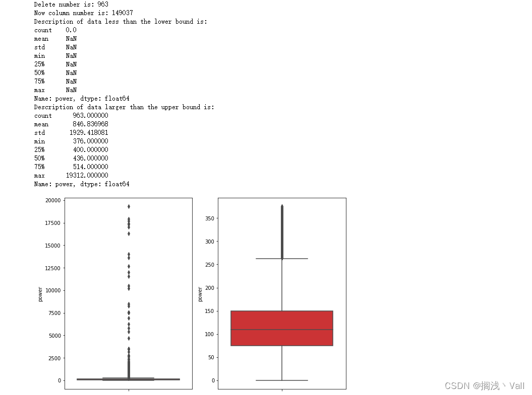
def outliers_proc(data, col_name, scale=3):
    """
    用于清洗异常值，默认用 box_plot（scale=3）进行清洗
    :param data: 接收 pandas 数据格式
    :param col_name: pandas 列名
    :param scale: 尺度
    :return:
    """

    def box_plot_outliers(data_ser, box_scale):
        """
        利用箱线图去除异常值
        :param data_ser: 接收 pandas.Series 数据格式
        :param box_scale: 箱线图尺度，
        :return:
        """
        iqr = box_scale * (data_ser.quantile(0.75) - data_ser.quantile(0.25))
        val_low = data_ser.quantile(0.25) - iqr
        val_up = data_ser.quantile(0.75) + iqr
        rule_low = (data_ser < val_low)
        rule_up = (data_ser > val_up)
        return (rule_low, rule_up), (val_low, val_up)

    data_n = data.copy()
    data_series = data_n[col_name]
    rule, value = box_plot_outliers(data_series, box_scale=scale)
    index = np.arange(data_series.shape[0])[rule[0] | rule[1]]
    print("Delete number is: {}".format(len(index)))
    data_n = data_n.drop(index)
    data_n.reset_index(drop=True, inplace=True)
    print("Now column number is: {}".format(data_n.shape[0]))
    index_low = np.arange(data_series.shape[0])[rule[0]]
    outliers = data_series.iloc[index_low]
    print("Description of data less than the lower bound is:")
    print(pd.Series(outliers).describe())
    index_up = np.arange(data_series.shape[0])[rule[1]]
    outliers = data_series.iloc[index_up]
    print("Description of data larger than the upper bound is:")
    print(pd.Series(outliers).describe())
    
    fig, ax = plt.subplots(1, 2, figsize=(10, 7))
    sns.boxplot(y=data[col_name], data=data, palette="Set1", ax=ax[0])
    sns.boxplot(y=data_n[col_name], data=data_n, palette="Set1", ax=ax[1])
    return data_n

# 我们可以删掉一些异常数据，以 power 为例。  
# 这里删不删同学可以自行判断
# 但是要注意 test 的数据不能删 = = 不能掩耳盗铃是不是
train = outliers_proc(train, 'power', scale=3)

# 训练集和测试集放在一起，方便构造特征
train['train']=1
test['train']=0
data = pd.concat([train, test], ignore_index=True, sort=False)
# 使用时间：data['creatDate'] - data['regDate']，反应汽车使用时间，一般来说价格与使用时间成反比
# 不过要注意，数据里有时间出错的格式，所以我们需要 errors='coerce'
data['used_time'] = (pd.to_datetime(data['creatDate'], format='%Y%m%d', errors='coerce') - 
                            pd.to_datetime(data['regDate'], format='%Y%m%d', errors='coerce')).dt.days
                            # 看一下空数据，有 15k 个样本的时间是有问题的，我们可以选择删除，也可以选择放着。
# 但是这里不建议删除，因为删除缺失数据占总样本量过大，7.5%
# 我们可以先放着，因为如果我们 XGBoost 之类的决策树，其本身就能处理缺失值，所以可以不用管；
data['used_time'].isnull().sum()
# 从邮编中提取城市信息，因为是德国的数据，所以参考德国的邮编，相当于加入了先验知识
data['city'] = data['regionCode'].apply(lambda x : str(x)[:-3])
# 计算某品牌的销售统计量，同学们还可以计算其他特征的统计量
# 这里要以 train 的数据计算统计量
train_gb = train.groupby("brand")
all_info = {}
for kind, kind_data in train_gb:
    info = {}
    kind_data = kind_data[kind_data['price'] > 0]
    info['brand_amount'] = len(kind_data)
    info['brand_price_max'] = kind_data.price.max()
    info['brand_price_median'] = kind_data.price.median()
    info['brand_price_min'] = kind_data.price.min()
    info['brand_price_sum'] = kind_data.price.sum()
    info['brand_price_std'] = kind_data.price.std()
    info['brand_price_average'] = round(kind_data.price.sum() / (len(kind_data) + 1), 2)
    all_info[kind] = info
brand_fe = pd.DataFrame(all_info).T.reset_index().rename(columns={"index": "brand"})
data = data.merge(brand_fe, how='left', on='brand')
# 数据分桶 以 power 为例
# 这时候我们的缺失值也进桶了，

# 数据分桶又叫数据分箱  
# 一般在建立分类模型时，需要对连续变量离散化，特征离散化后，模型会更稳定，降低了模型过拟合的风险。
#（1）常用的无监督分桶方法有等频分桶、等距分桶和聚类分桶。
#（2）有监督分桶主要有best-ks分桶和卡方分桶。

# 为什么要做数据分桶呢，原因有很多，= =
# 1. 离散后稀疏向量内积乘法运算速度更快，计算结果也方便存储，容易扩展；
# 2. 离散后的特征对异常值更具鲁棒性，如 age>30 为 1 否则为 0，对于年龄为 200 的也不会对模型造成很大的干扰；
# 3. LR 属于广义线性模型，表达能力有限，经过离散化后，每个变量有单独的权重，这相当于引入了非线性，能够提升模型的表达能力，加大拟合；
# 4. 离散后特征可以进行特征交叉，提升表达能力，由 M+N 个变量编程 M*N 个变量，进一步引入非线形，提升了表达能力；
# 5. 特征离散后模型更稳定，如用户年龄区间，不会因为用户年龄长了一岁就变化

# LightGBM是个快速的，分布式的，高性能的基于决策树算法的梯度提升框架。可用于排序，分类，回归以及很多其他的机器学习任务中。
# 当然还有很多原因，LightGBM 在改进 XGBoost 时就增加了数据分桶，增强了模型的泛化性

bin = [i*10 for i in range(31)]
data['power_bin'] = pd.cut(data['power'], bin, labels=False)
data[['power_bin', 'power']].head()
# 利用好了，就可以删掉原始数据了
data = data.drop(['creatDate', 'regDate', 'regionCode'], axis=1)
# 目前的数据其实已经可以给树模型使用了，所以我们导出一下
data.to_csv('data_for_tree.csv', index=0)

# 我们可以再构造一份特征给 LR NN 之类的模型用
# 之所以分开构造是因为，不同模型对数据集的要求不同
# 我们看下数据分布：
data['power'].plot.hist() # 绘制直方图
# 我们刚刚已经对 train 进行异常值处理了，但是现在还有这么奇怪的分布是因为 test 中的 power 异常值，
# 所以我们其实刚刚 train 中的 power 异常值不删为好，可以用长尾分布截断来代替
train['power'].plot.hist()
# 我们对其取 log，在做归一化
from sklearn import preprocessing
min_max_scaler = preprocessing.MinMaxScaler()
data['power'] = np.log(data['power'] + 1) 
data['power'] = ((data['power'] - np.min(data['power'])) / (np.max(data['power']) - np.min(data['power'])))
data['power'].plot.hist()
# km 的比较正常，应该是已经做过分桶了
data['kilometer'].plot.hist()
# 除此之外 还有我们刚刚构造的统计量特征：
# 'brand_amount', 'brand_price_average', 'brand_price_max',
# 'brand_price_median', 'brand_price_min', 'brand_price_std',
# 'brand_price_sum'
# 这里不再一一举例分析了，直接做变换，
def max_min(x):
    return (x - np.min(x)) / (np.max(x) - np.min(x))

data['brand_amount'] = ((data['brand_amount'] - np.min(data['brand_amount'])) / 
                        (np.max(data['brand_amount']) - np.min(data['brand_amount'])))
data['brand_price_average'] = ((data['brand_price_average'] - np.min(data['brand_price_average'])) / 
                               (np.max(data['brand_price_average']) - np.min(data['brand_price_average'])))
data['brand_price_max'] = ((data['brand_price_max'] - np.min(data['brand_price_max'])) / 
                           (np.max(data['brand_price_max']) - np.min(data['brand_price_max'])))
data['brand_price_median'] = ((data['brand_price_median'] - np.min(data['brand_price_median'])) /
                              (np.max(data['brand_price_median']) - np.min(data['brand_price_median'])))
data['brand_price_min'] = ((data['brand_price_min'] - np.min(data['brand_price_min'])) / 
                           (np.max(data['brand_price_min']) - np.min(data['brand_price_min'])))
data['brand_price_std'] = ((data['brand_price_std'] - np.min(data['brand_price_std'])) / 
                           (np.max(data['brand_price_std']) - np.min(data['brand_price_std'])))
data['brand_price_sum'] = ((data['brand_price_sum'] - np.min(data['brand_price_sum'])) / 
                           (np.max(data['brand_price_sum']) - np.min(data['brand_price_sum'])))
                           # 对类别特征进行 OneEncoder
data = pd.get_dummies(data, columns=['model', 'brand', 'bodyType', 'fuelType',
                                     'gearbox', 'notRepairedDamage', 'power_bin'])
                                     # 相关性分析
print(data['power'].corr(data['price'], method='spearman'))
print(data['kilometer'].corr(data['price'], method='spearman'))
print(data['brand_amount'].corr(data['price'], method='spearman'))
print(data['brand_price_average'].corr(data['price'], method='spearman'))
print(data['brand_price_max'].corr(data['price'], method='spearman'))
print(data['brand_price_median'].corr(data['price'], method='spearman'))
# 相关性分析可视化
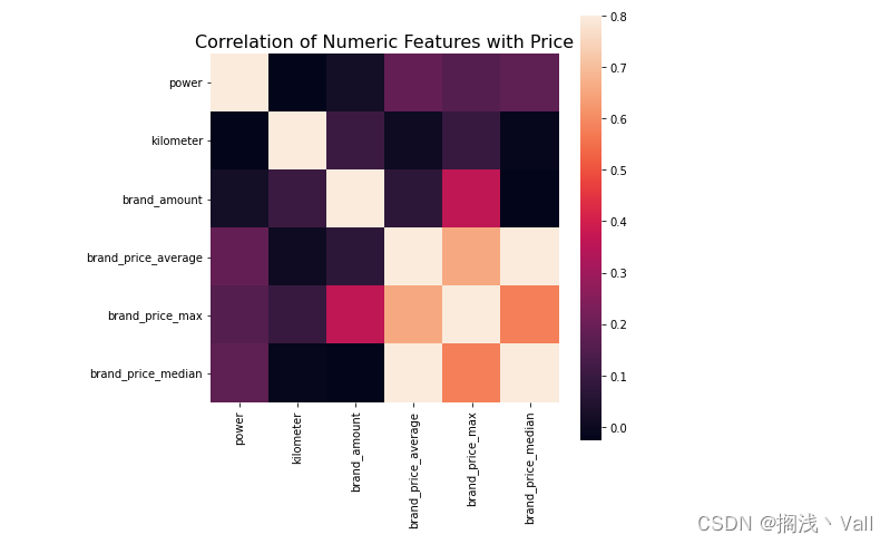
data_numeric = data[['power', 'kilometer', 'brand_amount', 'brand_price_average', 
                     'brand_price_max', 'brand_price_median']]
correlation = data_numeric.corr()

f , ax = plt.subplots(figsize = (7, 7))
plt.title('Correlation of Numeric Features with Price',y=1,size=16)
sns.heatmap(correlation,square = True,  vmax=0.8)
# 右下角的字段相关性高一些

!pip install mlxtend
# k_feature 太大会很难跑，没服务器，所以提前 interrupt 了
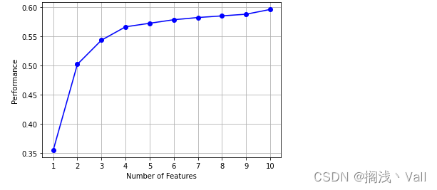
from mlxtend.feature_selection import SequentialFeatureSelector as SFS
from sklearn.linear_model import LinearRegression
sfs = SFS(LinearRegression(),
           k_features=10,
           forward=True,
           floating=False,
           scoring = 'r2',
           cv = 0)
x = data.drop(['price'], axis=1)
numerical_cols = x.select_dtypes(exclude = 'object').columns
x = x[numerical_cols]
x = x.fillna(0)
y = data['price'].fillna(0)
sfs.fit(x, y)
sfs.k_feature_names_ 
# 画出来，可以看到边际效益
from mlxtend.plotting import plot_sequential_feature_selection as plot_sfs
import matplotlib.pyplot as plt
fig1 = plot_sfs(sfs.get_metric_dict(), kind='std_dev')
plt.grid()
plt.show()