


 本文深入解析逻辑回归算法,从线性回归模型出发,通过sigmoid函数转换,形成适用于二分类问题的非线性模型。详细阐述了Logistic模型的数学原理,包括参数估计、损失函数及其梯度计算,并提供Python实现代码。
逻辑回归算法的Python实现
Logistic回归
原理浅析
Logistic逻辑回归是线性回归模型的一种函数映射,线性回归的预测是根据模型特征的线性叠加,在经过sigmoid函数之后模型就变成了非线性的,在x=0x=0x=0的时候梯度很高,在∣x∣|x|∣x∣越大时梯度越小。Logistic回归被用在二分类问题里面,其定义域为(0,1)(0,1)(0,1),在具体问题里面可以看做二分类的某一类的概率。
- 线性回归模型:
f(x)=w0+w1x1+...+wnxn=ΘTXf(x)=w_0 + w_1x_1+...+w_nx_n=\Theta^T{X}f(x)=w0+w1x1+...+wnxn=ΘTX
Θ=[w0w1w2⋯wn]\Theta=\begin{bmatrix}w_0&w_1&w_2&\cdots&w_n\end{bmatrix}Θ=[w0w1w2⋯wn],X=[1x1x2⋯xn]X=\begin{bmatrix}1&x_1&x_2&\cdots&x_n\end{bmatrix}X=[1x1x2⋯xn] - sigmod函数:
g(x)=11+e−xg(x)=\frac{1}{1+e^{-x}}g(x)=1+e−x1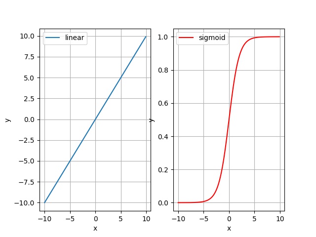
对于sigmoid函数来说,其单调可微,而且形似阶跃函数,xxx越大,yyy越趋近于1,xxx越小,yyy越趋近于0,这种变化就是logistic变化。
对于各个维度上面的特征来说,经过了线性模型再经过sigmoid函数,其Logistc模型为:
h(x)=g(f(x))=11+e−ΘTXh(x)=g(f(x))=\frac{1}{1+e^{-\Theta^TX}}h(x)=g(f(x))=1+e−ΘTX1
二分类问题使用sigmoid函数的原因为:
- 其定义域为概率分布的(0,1)(0,1)(0,1)
- 需要在因变量在sigmoid函数上面趋近于0的时候变化梯度,而不是线性变化
- 在形成损失函数之后形成凸函数
设正例为1,反例为0,在前向估计之后,可以得到:
{P(y=1∣x;θ)=hθ(x)P(y=0∣x;θ)=1−hθ(x)\begin{cases}
P(y=1|x;\theta)=h_\theta(x)\\
P(y=0|x;\theta)=1-h_\theta(x)\\
\end{cases}
{P(y=1∣x;θ)=hθ(x)P(y=0∣x;θ)=1−hθ(x)
可以简化为:
P(y∣x;θ)=(hθ(x))y(1−hθ(x))1−yP(y|x;\theta)=(h_\theta(x))^y(1-h_\theta(x))^{1-y}P(y∣x;θ)=(hθ(x))y(1−hθ(x))1−y
为了做参数估计,对其做最大似然估计:
L(θ)=∏i=1m(hθ(xi))yi(1−hθ(xi))1−yiL(\theta)=\prod_{i=1}^{m}(h_\theta(x^i))^{y^i}(1-h_\theta(x^i))^{1-y^i}L(θ)=i=1∏m(hθ(xi))yi(1−hθ(xi))1−yi
因为:
- 在求梯度的时候,连乘的直接微分相对复杂,可以使用log把连乘变成相加
- 概率值是浮点数,多个浮点数相乘易造成浮点数下溢,可以使用log把相乘变成相加
所以我们使用对数似然:
l(θ)=log(L(θ))=∑i=1myilog(hθ(xi))+(1−yi)log(1−hθ(xi))l(\theta)=log(L(\theta))=\sum_{i=1}^{m}y^ilog(h_\theta(x^i))+(1-y^i)log(1-h_\theta(x^i))l(θ)=log(L(θ))=i=1∑myilog(hθ(xi))+(1−yi)log(1−hθ(xi))
参数θ\thetaθ的梯度:
δl(θ)δ(θj)=∑i=1m(yihθ(xi)−1−yi1−hθ(xi))∙δ(hθ(xi))δθj=∑i=1m(yi−g(ΘTXi))∙xji\frac{\delta{}l(\theta)}{\delta(\theta_j)}=\sum_{i=1}^m\left(\frac{y^i}{h_\theta(x^i)} - \frac{1-y^i}{1-h_\theta(x^i)}\right)\bullet{}\frac{\delta(h_\theta(x^i))}{\delta\theta_j}=\sum_{i=1}^{m}(y^i-g(\Theta^TX^i))\bullet{}x_j^iδ(θj)δl(θ)=i=1∑m(hθ(xi)yi−1−hθ(xi)1−yi)∙δθjδ(hθ(xi))=i=1∑m(yi−g(ΘTXi))∙xji
将对数似然取负,那么得到的函数就可以当做损失函数:
loss=−∑i=1m[yilog(hθ(xi))+(1−yi)log(1−hθ(xi))]loss=-\sum_{i=1}^{m}[y^ilog(h_\theta(x^i))+(1-y^i)log(1-h_\theta(x^i))]loss=−i=1∑m[yilog(hθ(xi))+(1−yi)log(1−hθ(xi))]
参数θ\thetaθ的学习规则:
θj:=θj+α(yi−hθ(xi))xji\theta_j:=\theta_j+\alpha(y^i-h_\theta(x^i))x_j^iθj:=θj+α(yi−hθ(xi))xji
此时我们做的是随机梯度上升,α\alphaα是超参数,我们定义的学习率
为了防止过拟合,我们把损失函数加上正则项:
loss=−∑i=1m[yilog(hθ(xi))+(1−yi)log(1−hθ(xi))]+λ∑j=1nθj2loss=-\sum_{i=1}^{m}[y^ilog(h_\theta(x^i))+(1-y^i)log(1-h_\theta(x^i))]+\lambda\sum_{j=1}^n{\theta_j}^2loss=−i=1∑m[yilog(hθ(xi))+(1−yi)log(1−hθ(xi))]+λj=1∑nθj2
代码浅析
- 前向算法:
h(x)=11+e−ΘTXh(x)=\frac{1}{1+e^{-\Theta^TX}}h(x)=1+e−ΘTX1
其中XXX为xxx构成的特征矩阵,Θ\ThetaΘ是由www构成的参数矩阵# 前向预测算法 def forward_prediction(x, weights): f = np.matmul(x, weights.T) return np.divide(1, np.add(1, np.exp(-f))) - 损失函数:
loss=−∑i=1m(yilog(hw(xi))−∑i=1m(1−yi)log(1−hw(xi))+λ∑j=1nθj2loss=-\sum_{i=1}^{m}(y^ilog(h_w(x^i))-\sum_{i=1}^{m}(1-y^i)log(1-h_w(x^i))+\lambda\sum_{j=1}^n{\theta_j}^2loss=−i=1∑m(yilog(hw(xi))−i=1∑m(1−yi)log(1−hw(xi))+λj=1∑nθj2`
使用矩阵运算表示:
loss=1m[−YTlog(H)−((1−Y)T(1−H))+λLΘ2]loss=\frac{1}{m}[-Y^Tlog(H)-((1-Y)^T(1-H)) + \lambda{}L\Theta^2]loss=m1[−YTlog(H)−((1−Y)T(1−H))+λLΘ2]
其中λ\lambdaλ为超参数,λ\lambdaλ越小,越容易过拟合,越大,越容易欠拟合,LLL为对角矩阵# 带正则项的损失函数 def loss(weights, h, y, _lambda): count = y.shape[0] loss_1 = -np.matmul(y.T, np.log(h)) loss_0 = -np.matmul(np.add(1, -y).T, np.log(np.add(1, -h))) regularization_term = np.multiply(np.matmul(weights, weights.T), _lambda) loss_ = np.divide((loss_1 + loss_0 + regularization_term), count) return loss_ - 对于损失函数求导可得到各个参数的梯度:
δloss(θ)δθ=1m(XT(H−Y)+LΘ)\frac{\delta{}loss(\theta)}{\delta\theta}=\frac{1}{m}(X^T(H-Y)+L\Theta)δθδloss(θ)=m1(XT(H−Y)+LΘ)# 参数梯度 def gradient(x, h, y, alpha): count = h.shape[0] grad = np.divide(np.multiply(alpha, np.matmul(np.add(-y, h).T, x)), count) return grad
示例代码
# --*-- coding:utf8 --*--
import numpy as np
import matplotlib.pyplot as plt
def load_data():
data0, data1 = create_data()
data0 = np.append(data0, np.zeros((data0.shape[0], 1)), axis=1)
data1 = np.append(data1, np.ones((data1.shape[0], 1)), axis=1)
data = np.append(data0, data1, axis=0)
np.random.shuffle(data)
return data
# 制作数据
def create_data():
x_s = np.random.uniform(-1, 1, 1000)
y_s = [np.random.uniform(-limit, limit) for limit in np.sqrt(1 - np.square(x_s))]
x_1, y_1, x_2, y_2 = [], [], [], []
for i, x in enumerate(x_s):
if (x + y_s[i]) > x * y_s[i]:
x_1.append(x)
y_1.append(y_s[i])
else:
x_2.append(x)
y_2.append(y_s[i])
data0 = np.append(np.array([x_1]).T, np.array([y_1]).T, axis=1)
data1 = np.append(np.array([x_2]).T, np.array([y_2]).T, axis=1)
return data0, data1
# 前向预测算法
def forward_prediction(x, weights):
    f = np.matmul(x, weights.T)
    return np.divide(1, np.add(1, np.exp(-f)))
# 带正则项的损失函数
def loss(weights, h, y, _lambda):
  	count = y.shape[0]
  	loss_1 = -np.matmul(y.T, np.log(h))
  	loss_0 = -np.matmul(np.add(1, -y).T, np.log(np.add(1, -h)))
  	regularization_term = np.multiply(np.matmul(weights, weights.T), _lambda)
  	loss_ = np.divide((loss_1 + loss_0 + regularization_term), count)
  	return loss_
# 参数梯度
def gradient(x, h, y, alpha):
    count = h.shape[0]
    grad = np.divide(np.multiply(alpha, np.matmul(np.add(-y, h).T, x)), count)
    return grad
def main():
data = load_data()
x = data[:, :2]
y = np.array([data[:, 2]]).T
weights = np.zeros((1, x.shape[1]))
_lambda = 0.001
_alpha = 1
loss_arr = []
i = 1000
for _ in range(i):
h = forward_prediction(x=x, weights=weights)
_loss = loss(weights, h, y, _lambda)
grad = gradient(x, h, y, _alpha)
weights = weights - np.multiply(grad, _alpha)
loss_arr.append(_loss[0][0])
h = forward_prediction(x=x, weights=weights)
real = np.array([data[:, 2]]).T
_ = np.append(h, real, axis=1)
for __ in _:
print(__)
x_axis = np.arange(0, i, 1)
plt.plot(x_axis, loss_arr)
plt.show()
plt.draw()
if __name__ == '__main__':
main()


 3万+
3万+

 被折叠的 条评论
为什么被折叠?
被折叠的 条评论
为什么被折叠?
 到【灌水乐园】发言


