


12-1 Mnistinfogan
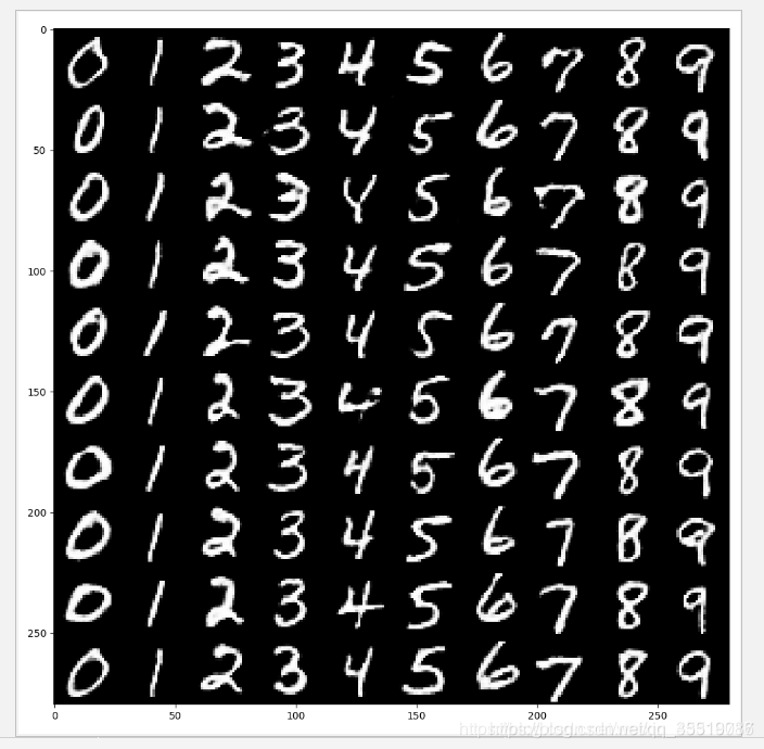
通过使用InfoGAN网络学习MNIST数据特征,生成以假乱真的MNIST模拟样本,并发现内部潜在的特征信息。
程序:
#1 引入头文件并加载MNIST数据
import numpy as np
import tensorflow as tf
import matplotlib.pyplot as plt
from scipy.stats import norm
import tensorflow.contrib.slim as slim

from tensorflow.examples.tutorials.mnist import input_data

mnist = input_data.read_data_sets("/data/")  # , one_hot=True)

tf.reset_default_graph()#用于清除默认图形堆栈并重置全局默认图形
'''------------------------------------------------------'''
#3 定义生成器与判别器

def generator(x):
    reuse = len([t for t in tf.global_variables() if t.name.startswith('generator')]) > 0
    # print (x.get_shape())
    with tf.variable_scope('generator', reuse=reuse):
        x = slim.fully_connected(x, 1024)
        # print( x)
        x = slim.batch_norm(x, activation_fn=tf.nn.relu)
        x = slim.fully_connected(x, 7 * 7 * 128)
        x = slim.batch_norm(x, activation_fn=tf.nn.relu)
        x = tf.reshape(x, [-1, 7, 7, 128])
        # print '22',tensor.get_shape()
        x = slim.conv2d_transpose(x, 64, kernel_size=[4, 4], stride=2, activation_fn=None)
        # print ('gen',x.get_shape())
        x = slim.batch_norm(x, activation_fn=tf.nn.relu)
        z = slim.conv2d_transpose(x, 1, kernel_size=[4, 4], stride=2, activation_fn=tf.nn.sigmoid)
        # print ('genz',z.get_shape())
    return z


def leaky_relu(x):
    return tf.where(tf.greater(x, 0), x, 0.01 * x)


def discriminator(x, num_classes=10, num_cont=2):#判别函数
    reuse = len([t for t in tf.global_variables() if t.name.startswith('discriminator')]) > 0
    # print (reuse)
    # print (x.get_shape())
    with tf.variable_scope('discriminator', reuse=reuse):
        x = tf.reshape(x, shape=[-1, 28, 28, 1])
        x = slim.conv2d(x, num_outputs=64, kernel_size=[4, 4], stride=2, activation_fn=leaky_relu)
        x = slim.conv2d(x, num_outputs=128, kernel_size=[4, 4], stride=2, activation_fn=leaky_relu)
        # print ("conv2d",x.get_shape())
        x = slim.flatten(x)
        shared_tensor = slim.fully_connected(x, num_outputs=1024, activation_fn=leaky_relu)
        recog_shared = slim.fully_connected(shared_tensor, num_outputs=128, activation_fn=leaky_relu)
        disc = slim.fully_connected(shared_tensor, num_outputs=1, activation_fn=None)
        disc = tf.squeeze(disc, -1)
        # print ("disc",disc.get_shape())#0 or 1
        recog_cat = slim.fully_connected(recog_shared, num_outputs=num_classes, activation_fn=None)
        recog_cont = slim.fully_connected(recog_shared, num_outputs=num_cont, activation_fn=tf.nn.sigmoid)
    return disc, recog_cat, recog_cont
'''------------------------------------------------------'''
#4 定义网络模型

batch_size = 10  # 获取样本的批次大小32
classes_dim = 10  # 10 classes
con_dim = 2  #隐含信息变量的维度 total continuous factor
rand_dim = 38
n_input = 784

x = tf.placeholder(tf.float32, [None, n_input])
y = tf.placeholder(tf.int32, [None])

z_con = tf.random_normal((batch_size, con_dim))  # 2列
z_rand = tf.random_normal((batch_size, rand_dim))  # 38列
z = tf.concat(axis=1, values=[tf.one_hot(y, depth=classes_dim), z_con, z_rand])  # 50列
gen = generator(z)
genout = tf.squeeze(gen, -1)

# labels for discriminator
y_real = tf.ones(batch_size)  # 真
y_fake = tf.zeros(batch_size)  # 假

# 判别器
disc_real, class_real, _ = discriminator(x)#真样本的输出
disc_fake, class_fake, con_fake = discriminator(gen)#模拟样本的输出
pred_class = tf.argmax(class_fake, dimension=1)
'''------------------------------------------------------'''
#5 定义损失函数与优化器

# 判别器 loss
loss_d_r = tf.reduce_mean(tf.nn.sigmoid_cross_entropy_with_logits(logits=disc_real, labels=y_real))
loss_d_f = tf.reduce_mean(tf.nn.sigmoid_cross_entropy_with_logits(logits=disc_fake, labels=y_fake))
loss_d = (loss_d_r + loss_d_f) / 2
# print ('loss_d', loss_d.get_shape())
# generator loss
loss_g = tf.reduce_mean(tf.nn.sigmoid_cross_entropy_with_logits(logits=disc_fake, labels=y_real))
# categorical factor loss
loss_cf = tf.reduce_mean(tf.nn.sparse_softmax_cross_entropy_with_logits(logits=class_fake, labels=y))  # class ok 图片对不上
loss_cr = tf.reduce_mean(
    tf.nn.sparse_softmax_cross_entropy_with_logits(logits=class_real, labels=y))  # 生成的图片与class ok 与输入的class对不上
loss_c = (loss_cf + loss_cr) / 2
#隐含信息变量的loss continuous factor loss
loss_con = tf.reduce_mean(tf.square(con_fake - z_con))

# 获得各个网络中各自的训练参数
t_vars = tf.trainable_variables()
d_vars = [var for var in t_vars if 'discriminator' in var.name]
g_vars = [var for var in t_vars if 'generator' in var.name]

disc_global_step = tf.Variable(0, trainable=False)
gen_global_step = tf.Variable(0, trainable=False)

train_disc = tf.train.AdamOptimizer(0.0001).minimize(loss_d + loss_c + loss_con, var_list=d_vars,
                                                     global_step=disc_global_step)
train_gen = tf.train.AdamOptimizer(0.001).minimize(loss_g + loss_c + loss_con, var_list=g_vars,
                                                   global_step=gen_global_step)
'''------------------------------------------------------'''
#6 开始训练与测试

training_epochs = 3
display_step = 1

with tf.Session() as sess:
    sess.run(tf.global_variables_initializer())

    for epoch in range(training_epochs):
        avg_cost = 0.
        total_batch = int(mnist.train.num_examples / batch_size)

        # 遍历全部数据集
        for i in range(total_batch):
            batch_xs, batch_ys = mnist.train.next_batch(batch_size)  # 取数据
            feeds = {x: batch_xs, y: batch_ys}

            # Fit training using batch data
            l_disc, _, l_d_step = sess.run([loss_d, train_disc, disc_global_step], feeds)
            l_gen, _, l_g_step = sess.run([loss_g, train_gen, gen_global_step], feeds)

        # 显示训练中的详细信息
        if epoch % display_step == 0:
            print("Epoch:", '%04d' % (epoch + 1), "cost=", "{:.9f} ".format(l_disc), l_gen)

    print("完成!")

    # 测试
    print ("Result:", loss_d.eval({x: mnist.test.images[:batch_size], y: mnist.test.labels[:batch_size]})
           , loss_g.eval({x: mnist.test.images[:batch_size], y: mnist.test.labels[:batch_size]}))

    '''------------------------------------------------------'''
    #7 可视化

    # 根据图片模拟生成图片
    show_num = 10
    gensimple, d_class, inputx, inputy, con_out = sess.run(
        [genout, pred_class, x, y, con_fake],
        feed_dict={x: mnist.test.images[:batch_size], y: mnist.test.labels[:batch_size]})

    f, a = plt.subplots(2, 10, figsize=(10, 2))
    for i in range(show_num):
        a[0][i].imshow(np.reshape(inputx[i], (28, 28)))
        a[1][i].imshow(np.reshape(gensimple[i], (28, 28)))
        print("d_class", d_class[i], "inputy", inputy[i], "con_out", con_out[i])

    plt.draw()
    plt.show()

    my_con = tf.placeholder(tf.float32, [batch_size, 2])
    myz = tf.concat(axis=1, values=[tf.one_hot(y, depth=classes_dim), my_con, z_rand])
    mygen = generator(myz)
    mygenout = tf.squeeze(mygen, -1)

    my_con1 = np.ones([10, 2])
    a = np.linspace(0.0001, 0.99999, 10)
    y_input = np.ones([10])
    figure = np.zeros((28 * 10, 28 * 10))
    my_rand = tf.random_normal((10, rand_dim))
    for i in range(10):
        for j in range(10):
            my_con1[j][0] = a[i]
            my_con1[j][1] = a[j]
            y_input[j] = j
        mygenoutv = sess.run(mygenout, feed_dict={y: y_input, my_con: my_con1})
        for jj in range(10):
            digit = mygenoutv[jj].reshape(28, 28)
            figure[i * 28: (i + 1) * 28,
            jj * 28: (jj + 1) * 28] = digit

    plt.figure(figsize=(10, 10))
    plt.imshow(figure, cmap='Greys_r')
    plt.show()
结果:
Extracting /data/train-images-idx3-ubyte.gz
Extracting /data/train-labels-idx1-ubyte.gz
Extracting /data/t10k-images-idx3-ubyte.gz
Extracting /data/t10k-labels-idx1-ubyte.gz

Epoch: 0001 cost= 0.746451676  0.764629
Epoch: 0002 cost= 0.646678686  0.9203032
Epoch: 0003 cost= 0.516349673  0.8423565
完成!
Result: 0.47129387 0.97945136
d_class 7 inputy 7 con_out [0.00358483 0.34325057]
d_class 2 inputy 2 con_out [9.9193072e-01 2.1791458e-04]
d_class 1 inputy 1 con_out [3.1650066e-05 1.6704202e-04]
d_class 0 inputy 0 con_out [0.98508525 0.6656839 ]
d_class 4 inputy 4 con_out [0.02977383 0.00412542]
d_class 1 inputy 1 con_out [0.02095369 0.04388431]
d_class 4 inputy 4 con_out [7.5429678e-05 1.8178523e-03]
d_class 9 inputy 9 con_out [0.20877889 0.9998402 ]
d_class 5 inputy 5 con_out [0.99537027 0.01209643]
d_class 9 inputy 9 con_out [0.13495213 0.0034132 ]

12-2 aegan
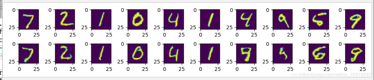
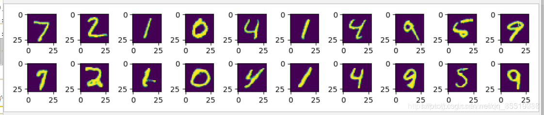
通过使用前面的InfoGAN网络例子,在其基础上添加自编码网络,将InfoGAN的参数固定,训练反向生成器(自编码网络中的编码器),并将生成的模型用于MNIST数据集样本重建,得到相似样本。
程序:
import numpy as np
import tensorflow as tf
import matplotlib.pyplot as plt
from scipy.stats import norm
import tensorflow.contrib.slim as slim

from tensorflow.examples.tutorials.mnist import input_data

mnist = input_data.read_data_sets("/data/")  # , one_hot=True)

tf.reset_default_graph()


# 生成器函数
def generator(x):
    reuse = len([t for t in tf.global_variables() if t.name.startswith('generator')]) > 0
    with tf.variable_scope('generator', reuse=reuse):
        # 两个带bn的全连接
        x = slim.fully_connected(x, 1024)
        x = slim.batch_norm(x, activation_fn=tf.nn.relu)
        x = slim.fully_connected(x, 7 * 7 * 128)
        x = slim.batch_norm(x, activation_fn=tf.nn.relu)
        # 两个转置卷积
        x = tf.reshape(x, [-1, 7, 7, 128])
        x = slim.conv2d_transpose(x, 64, kernel_size=[4, 4], stride=2, activation_fn=None)
        x = slim.batch_norm(x, activation_fn=tf.nn.relu)
        z = slim.conv2d_transpose(x, 1, kernel_size=[4, 4], stride=2, activation_fn=tf.nn.sigmoid)
    return z
'''--------------------------------------------------------'''
#1 添加反向生成器

# 反向生成器定义,结构与判别器类似
def inversegenerator(x):
    reuse = len([t for t in tf.global_variables() if t.name.startswith('inversegenerator')]) > 0
    with tf.variable_scope('inversegenerator', reuse=reuse):
        # 两个卷积
        x = tf.reshape(x, shape=[-1, 28, 28, 1])
        x = slim.conv2d(x, num_outputs=64, kernel_size=[4, 4], stride=2, activation_fn=leaky_relu)
        x = slim.conv2d(x, num_outputs=128, kernel_size=[4, 4], stride=2, activation_fn=leaky_relu)
        # 两个全连接
        x = slim.flatten(x)
        shared_tensor = slim.fully_connected(x, num_outputs=1024, activation_fn=leaky_relu)
        z = slim.fully_connected(shared_tensor, num_outputs=50, activation_fn=leaky_relu)
    return z
'''--------------------------------------------------------'''


# leaky relu定义
def leaky_relu(x):
    return tf.where(tf.greater(x, 0), x, 0.01 * x)


# 判别器定义
def discriminator(x, num_classes=10, num_cont=2):
    reuse = len([t for t in tf.global_variables() if t.name.startswith('discriminator')]) > 0

    with tf.variable_scope('discriminator', reuse=reuse):
        # 两个卷积
        x = tf.reshape(x, shape=[-1, 28, 28, 1])
        x = slim.conv2d(x, num_outputs=64, kernel_size=[4, 4], stride=2, activation_fn=leaky_relu)
        x = slim.conv2d(x, num_outputs=128, kernel_size=[4, 4], stride=2, activation_fn=leaky_relu)
        # print ("conv2d",x.get_shape())
        x = slim.flatten(x)
        # 两个全连接
        shared_tensor = slim.fully_connected(x, num_outputs=1024, activation_fn=leaky_relu)
        recog_shared = slim.fully_connected(shared_tensor, num_outputs=128, activation_fn=leaky_relu)
        # 通过全连接变换,生成输出信息。
        disc = slim.fully_connected(shared_tensor, num_outputs=1, activation_fn=None)
        disc = tf.squeeze(disc, -1)
        # print ("disc",disc.get_shape())#0 or 1
        recog_cat = slim.fully_connected(recog_shared, num_outputs=num_classes, activation_fn=None)
        recog_cont = slim.fully_connected(recog_shared, num_outputs=num_cont, activation_fn=tf.nn.sigmoid)
    return disc, recog_cat, recog_cont


batch_size = 10  # 最小批次
classes_dim = 10  # 10类数字
con_dim = 2  # total continuous factor
rand_dim = 38
n_input = 784

x = tf.placeholder(tf.float32, [None, n_input])
y = tf.placeholder(tf.int32, [None])

z_con = tf.random_normal((batch_size, con_dim))  # 2列
z_rand = tf.random_normal((batch_size, rand_dim))  # 38列
z = tf.concat(axis=1, values=[tf.one_hot(y, depth=classes_dim), z_con, z_rand])  # 50列
'''--------------------------------------------------------'''
#2 添加自编码网络代码

gen = generator(z)
genout = tf.squeeze(gen, -1)

# 自编码网络
aelearning_rate = 0.01
igen = generator(inversegenerator(generator(z)))
loss_ae = tf.reduce_mean(tf.pow(gen - igen, 2))

# 输出
igenout = generator(inversegenerator(x))

# 判别器结果标签 labels for discriminator
y_real = tf.ones(batch_size)  # 真
y_fake = tf.zeros(batch_size)  # 假
'''--------------------------------------------------------'''

# 判别器
disc_real, class_real, _ = discriminator(x)
disc_fake, class_fake, con_fake = discriminator(gen)
pred_class = tf.argmax(class_fake, dimension=1)

# 判别器 loss
loss_d_r = tf.reduce_mean(tf.nn.sigmoid_cross_entropy_with_logits(logits=disc_real, labels=y_real))
loss_d_f = tf.reduce_mean(tf.nn.sigmoid_cross_entropy_with_logits(logits=disc_fake, labels=y_fake))
loss_d = (loss_d_r + loss_d_f) / 2

# generator loss
loss_g = tf.reduce_mean(tf.nn.sigmoid_cross_entropy_with_logits(logits=disc_fake, labels=y_real))
# categorical factor loss
loss_cf = tf.reduce_mean(tf.nn.sparse_softmax_cross_entropy_with_logits(logits=class_fake, labels=y))  # class ok 图片对不上
loss_cr = tf.reduce_mean(
    tf.nn.sparse_softmax_cross_entropy_with_logits(logits=class_real, labels=y))  # 生成的图片与class ok 与输入的class对不上
loss_c = (loss_cf + loss_cr) / 2
# continuous factor loss
loss_con = tf.reduce_mean(tf.square(con_fake - z_con))
'''--------------------------------------------------------'''
#3 添加自编码网络的训练参数列表,定义优化器

# 获得各个网络中各自的训练参数
t_vars = tf.trainable_variables()
d_vars = [var for var in t_vars if 'discriminator' in var.name]
g_vars = [var for var in t_vars if 'generator' in var.name]
ae_vars = [var for var in t_vars if 'inversegenerator' in var.name]

# disc_global_step = tf.Variable(0, trainable=False)
gen_global_step = tf.Variable(0, trainable=False)
# ae_global_step = tf.Variable(0, trainable=False)
global_step = tf.train.get_or_create_global_step()  # 使用MonitoredTrainingSession,必须有

train_disc = tf.train.AdamOptimizer(0.0001).minimize(loss_d + loss_c + loss_con, var_list=d_vars,
                                                     global_step=global_step)
train_gen = tf.train.AdamOptimizer(0.001).minimize(loss_g + loss_c + loss_con, var_list=g_vars,
                                                   global_step=gen_global_step)
train_ae = tf.train.AdamOptimizer(aelearning_rate).minimize(loss_ae, var_list=ae_vars, global_step=global_step)

training_GANepochs = 3  # 训练GAN迭代3次数据集
training_aeepochs = 6  # 训练AE迭代3次数据集(从3开始到6)
'''--------------------------------------------------------'''

display_step = 1
'''--------------------------------------------------------'''
#4 启动session依次训练GAN与AE网络

with tf.train.MonitoredTrainingSession(checkpoint_dir='log/aecheckpoints', save_checkpoint_secs=120) as sess:
    total_batch = int(mnist.train.num_examples / batch_size)
    print("ae_global_step.eval(session=sess)", global_step.eval(session=sess),
          int(global_step.eval(session=sess) / total_batch))

    for epoch in range(int(global_step.eval(session=sess) / total_batch), training_GANepochs):
        avg_cost = 0.

        # 遍历全部数据集
        for i in range(total_batch):
            batch_xs, batch_ys = mnist.train.next_batch(batch_size)  # 取数据
            feeds = {x: batch_xs, y: batch_ys}

            # Fit training using batch data
            l_disc, _, l_d_step = sess.run([loss_d, train_disc, global_step], feeds)
            l_gen, _, l_g_step = sess.run([loss_g, train_gen, gen_global_step], feeds)

        # 显示训练中的详细信息
        if epoch % display_step == 0:
            print("Epoch:", '%04d' % (epoch + 1), "cost=", "{:.9f} ".format(l_disc), l_gen)

    print("GAN完成!")
    # 测试
    print("Result:", loss_d.eval({x: mnist.test.images[:batch_size], y: mnist.test.labels[:batch_size]}, session=sess)
          , loss_g.eval({x: mnist.test.images[:batch_size], y: mnist.test.labels[:batch_size]}, session=sess))

    # 根据图片模拟生成图片
    show_num = 10
    gensimple, inputx = sess.run(
        [genout, x], feed_dict={x: mnist.test.images[:batch_size], y: mnist.test.labels[:batch_size]})

    f, a = plt.subplots(2, 10, figsize=(10, 2))
    for i in range(show_num):
        a[0][i].imshow(np.reshape(inputx[i], (28, 28)))
        a[1][i].imshow(np.reshape(gensimple[i], (28, 28)))

    plt.draw()
    plt.show()

    # begin ae
    print("ae_global_step.eval(session=sess)", global_step.eval(session=sess),
          int(global_step.eval(session=sess) / total_batch))
    for epoch in range(int(global_step.eval(session=sess) / total_batch), training_aeepochs):
        avg_cost = 0.

        # 遍历全部数据集
        for i in range(total_batch):
            batch_xs, batch_ys = mnist.train.next_batch(batch_size)  # 取数据
            feeds = {x: batch_xs, y: batch_ys}

            # Fit training using batch data
            l_ae, _, ae_step = sess.run([loss_ae, train_ae, global_step], feeds)

        # 显示训练中的详细信息
        if epoch % display_step == 0:
            print("Epoch:", '%04d' % (epoch + 1), "cost=", "{:.9f} ".format(l_ae))

    # 测试
    print("Result:", loss_ae.eval({x: mnist.test.images[:batch_size], y: mnist.test.labels[:batch_size]}, session=sess))

    # 根据图片模拟生成图片
    show_num = 10
    gensimple, inputx = sess.run(
        [igenout, x], feed_dict={x: mnist.test.images[:batch_size], y: mnist.test.labels[:batch_size]})

    f, a = plt.subplots(2, 10, figsize=(10, 2))
    for i in range(show_num):
        a[0][i].imshow(np.reshape(inputx[i], (28, 28)))
        a[1][i].imshow(np.reshape(gensimple[i], (28, 28)))

    plt.draw()
    plt.show()
结果:
Extracting /data/train-images-idx3-ubyte.gz
Extracting /data/train-labels-idx1-ubyte.gz
Extracting /data/t10k-images-idx3-ubyte.gz
Extracting /data/t10k-labels-idx1-ubyte.gz

ae_global_step.eval(session=sess) 0 0
Epoch: 0001 cost= 0.576281667  0.84093344
Epoch: 0002 cost= 0.599554658  1.0545613
Epoch: 0003 cost= 0.584393144  0.7366768
GAN完成!
Result: 0.7863022 0.7851018
ae_global_step.eval(session=sess) 16500 3
Epoch: 0004 cost= 0.028643085
Epoch: 0005 cost= 0.036065791
Epoch: 0006 cost= 0.022045245
Result: 0.02327577
GAN结果:

AEGAN结果:
12.3 构建WGAN-GP生成MNIST数据集
通过使用WGAN-GP网络学习MNIST数据特征,并生成以假乱真的MNIST模拟样本。
程序:
import tensorflow as tf
from tensorflow.examples.tutorials.mnist import input_data
import os
import numpy as np
from scipy import misc, ndimage
import tensorflow.contrib.slim as slim

# from tensorflow.python.ops import init_ops

mnist = input_data.read_data_sets("/data/", one_hot=True)

batch_size = 100
width, height = 28, 28
mnist_dim = 784
random_dim = 10

tf.reset_default_graph()


def G(x):
    reuse = len([t for t in tf.global_variables() if t.name.startswith('generator')]) > 0
    with tf.variable_scope('generator', reuse=reuse):
        x = slim.fully_connected(x, 32, activation_fn=tf.nn.relu)
        x = slim.fully_connected(x, 128, activation_fn=tf.nn.relu)
        x = slim.fully_connected(x, mnist_dim, activation_fn=tf.nn.sigmoid)
    return x


def D(X):
    reuse = len([t for t in tf.global_variables() if t.name.startswith('discriminator')]) > 0
    with tf.variable_scope('discriminator', reuse=reuse):
        X = slim.fully_connected(X, 128, activation_fn=tf.nn.relu)
        X = slim.fully_connected(X, 32, activation_fn=tf.nn.relu)
        X = slim.fully_connected(X, 1, activation_fn=None)
    return X


real_X = tf.placeholder(tf.float32, shape=[batch_size, mnist_dim])
random_X = tf.placeholder(tf.float32, shape=[batch_size, random_dim])
random_Y = G(random_X)

eps = tf.random_uniform([batch_size, 1], minval=0., maxval=1.)
X_inter = eps * real_X + (1. - eps) * random_Y
grad = tf.gradients(D(X_inter), [X_inter])[0]
grad_norm = tf.sqrt(tf.reduce_sum((grad) ** 2, axis=1))
grad_pen = 10 * tf.reduce_mean(tf.nn.relu(grad_norm - 1.))

D_loss = tf.reduce_mean(D(random_Y)) - tf.reduce_mean(D(real_X)) + grad_pen
G_loss = -tf.reduce_mean(D(random_Y))

# 获得各个网络中各自的训练参数
t_vars = tf.trainable_variables()
d_vars = [var for var in t_vars if 'discriminator' in var.name]
g_vars = [var for var in t_vars if 'generator' in var.name]
print(len(t_vars), len(d_vars))

D_solver = tf.train.AdamOptimizer(1e-4, 0.5).minimize(D_loss, var_list=d_vars)
G_solver = tf.train.AdamOptimizer(1e-4, 0.5).minimize(G_loss, var_list=g_vars)

training_epochs = 100

with tf.Session() as sess:
    sess.run(tf.global_variables_initializer())
    if not os.path.exists('out/'):
        os.makedirs('out/')

    for epoch in range(training_epochs):

        total_batch = int(mnist.train.num_examples / batch_size)

        # 遍历全部数据集
        for e in range(total_batch):
            for i in range(5):
                real_batch_X, _ = mnist.train.next_batch(batch_size)
                random_batch_X = np.random.uniform(-1, 1, (batch_size, random_dim))
                _, D_loss_ = sess.run([D_solver, D_loss], feed_dict={real_X: real_batch_X, random_X: random_batch_X})

            random_batch_X = np.random.uniform(-1, 1, (batch_size, random_dim))
            _, G_loss_ = sess.run([G_solver, G_loss], feed_dict={random_X: random_batch_X})

        if epoch % 10 == 0:
            print('epoch %s, D_loss: %s, G_loss: %s' % (epoch, D_loss_, G_loss_))
            n_rows = 6
            check_imgs = sess.run(random_Y, feed_dict={random_X: random_batch_X}).reshape((batch_size, width, height))[
                         :n_rows * n_rows]
            imgs = np.ones((width * n_rows + 5 * n_rows + 5, height * n_rows + 5 * n_rows + 5))
            # print(np.shape(imgs))#(203, 203)

            for i in range(n_rows * n_rows):
                num1 = (i % n_rows)
                num2 = np.int32(i / n_rows)
                imgs[5 + 5 * num1 + width * num1:5 + 5 * num1 + width + width * num1,
                5 + 5 * num2 + height * num2:5 + 5 * num2 + height + height * num2] = check_imgs[i]

            misc.imsave('out/%s.png' % (epoch / 10), imgs)

    print("完成!")
结果:
epoch 0, D_loss: -4.3674254, G_loss: 0.42139548
epoch 10, D_loss: -2.1357408, G_loss: 1.2864103
epoch 20, D_loss: -2.408492, G_loss: 1.4262085
epoch 30, D_loss: -1.9260483, G_loss: 1.6472778
epoch 40, D_loss: -1.5441133, G_loss: 1.4730612
epoch 50, D_loss: -1.3460733, G_loss: 1.2684302
epoch 60, D_loss: -1.2566698, G_loss: 1.4221616
epoch 70, D_loss: -1.1435932, G_loss: 1.5208447
epoch 80, D_loss: -1.0484169, G_loss: 1.6984334
epoch 90, D_loss: -1.1097151, G_loss: 1.6389039
完成!
12-4 mnistLSgan
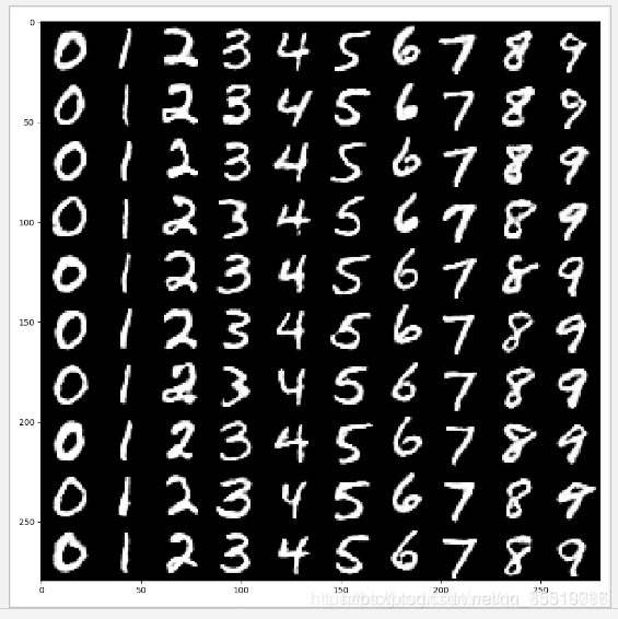
通过使用LSGAN网络学习MNIST数据特征,并生成以假乱真的MNIST模拟样本。
程序:
import numpy as np
import tensorflow as tf
import matplotlib.pyplot as plt
from scipy.stats import norm
import tensorflow.contrib.slim as slim

from tensorflow.examples.tutorials.mnist import input_data

mnist = input_data.read_data_sets("/data/")  # , one_hot=True)

tf.reset_default_graph()


def generator(x):
    reuse = len([t for t in tf.global_variables() if t.name.startswith('generator')]) > 0
    # print (x.get_shape())
    with tf.variable_scope('generator', reuse=reuse):
        x = slim.fully_connected(x, 1024)
        # print( x)
        x = slim.batch_norm(x, activation_fn=tf.nn.relu)
        x = slim.fully_connected(x, 7 * 7 * 128)
        x = slim.batch_norm(x, activation_fn=tf.nn.relu)
        x = tf.reshape(x, [-1, 7, 7, 128])
        # print '22',tensor.get_shape()
        x = slim.conv2d_transpose(x, 64, kernel_size=[4, 4], stride=2, activation_fn=None)
        # print ('gen',x.get_shape())
        x = slim.batch_norm(x, activation_fn=tf.nn.relu)
        z = slim.conv2d_transpose(x, 1, kernel_size=[4, 4], stride=2, activation_fn=tf.nn.sigmoid)
        # print ('genz',z.get_shape())
    return z


def leaky_relu(x):
    return tf.where(tf.greater(x, 0), x, 0.01 * x)
'''-----------------------------------------------'''
#1 修改判别器

def discriminator(x, num_classes=10, num_cont=2):
    reuse = len([t for t in tf.global_variables() if t.name.startswith('discriminator')]) > 0
    # print (reuse)
    # print (x.get_shape())
    with tf.variable_scope('discriminator', reuse=reuse):
        x = tf.reshape(x, shape=[-1, 28, 28, 1])
        x = slim.conv2d(x, num_outputs=64, kernel_size=[4, 4], stride=2, activation_fn=leaky_relu)
        x = slim.conv2d(x, num_outputs=128, kernel_size=[4, 4], stride=2, activation_fn=leaky_relu)
        # print ("conv2d",x.get_shape())
        x = slim.flatten(x)
        shared_tensor = slim.fully_connected(x, num_outputs=1024, activation_fn=leaky_relu)
        recog_shared = slim.fully_connected(shared_tensor, num_outputs=128, activation_fn=leaky_relu)
        disc = slim.fully_connected(shared_tensor, num_outputs=1, activation_fn=tf.nn.sigmoid)
        disc = tf.squeeze(disc, -1)
        # print ("disc",disc.get_shape())#0 or 1
        recog_cat = slim.fully_connected(recog_shared, num_outputs=num_classes, activation_fn=None)
        recog_cont = slim.fully_connected(recog_shared, num_outputs=num_cont, activation_fn=tf.nn.sigmoid)
    return disc, recog_cat, recog_cont
'''-----------------------------------------------'''

batch_size = 10  # 获取样本的批次大小32
classes_dim = 10  # 10 classes
con_dim = 2  # total continuous factor
rand_dim = 38
n_input = 784

x = tf.placeholder(tf.float32, [None, n_input])
y = tf.placeholder(tf.int32, [None])

z_con = tf.random_normal((batch_size, con_dim))  # 2列
z_rand = tf.random_normal((batch_size, rand_dim))  # 38列
z = tf.concat(axis=1, values=[tf.one_hot(y, depth=classes_dim), z_con, z_rand])  # 50列
gen = generator(z)
genout = tf.squeeze(gen, -1)

# labels for discriminator
# y_real = tf.ones(batch_size) #真
# y_fake = tf.zeros(batch_size)#假
'''-----------------------------------------------'''
#2 修改loss值

# 判别器
disc_real, class_real, _ = discriminator(x)
disc_fake, class_fake, con_fake = discriminator(gen)
pred_class = tf.argmax(class_fake, dimension=1)

# 判别器 loss
# loss_d_r = tf.reduce_mean(tf.nn.sigmoid_cross_entropy_with_logits(logits=disc_real, labels=y_real))
# loss_d_f = tf.reduce_mean(tf.nn.sigmoid_cross_entropy_with_logits(logits=disc_fake, labels=y_fake))
# loss_d = (loss_d_r + loss_d_f) / 2
# 最小乘二loss
loss_d = tf.reduce_sum(tf.square(disc_real - 1) + tf.square(disc_fake)) / 2
loss_g = tf.reduce_sum(tf.square(disc_fake - 1)) / 2
'''-----------------------------------------------'''

# generator loss
# loss_g = tf.reduce_mean(tf.nn.sigmoid_cross_entropy_with_logits(logits=disc_fake, labels=y_real))
# categorical factor loss
loss_cf = tf.reduce_mean(tf.nn.sparse_softmax_cross_entropy_with_logits(logits=class_fake, labels=y))  # class ok 图片对不上
loss_cr = tf.reduce_mean(tf.nn.sparse_softmax_cross_entropy_with_logits(logits=class_real, labels=y))  # 生成的图片与class ok 与输入的class对不上
loss_c = (loss_cf + loss_cr) / 2
# continuous factor loss
loss_con = tf.reduce_mean(tf.square(con_fake - z_con))

# 获得各个网络中各自的训练参数
t_vars = tf.trainable_variables()
d_vars = [var for var in t_vars if 'discriminator' in var.name]
g_vars = [var for var in t_vars if 'generator' in var.name]

disc_global_step = tf.Variable(0, trainable=False)
gen_global_step = tf.Variable(0, trainable=False)

train_disc = tf.train.AdamOptimizer(0.0001).minimize(loss_d + loss_c + loss_con, var_list=d_vars,
                                                     global_step=disc_global_step)
train_gen = tf.train.AdamOptimizer(0.001).minimize(loss_g + loss_c + loss_con, var_list=g_vars,
                                                   global_step=gen_global_step)

training_epochs = 3
display_step = 1
'''-----------------------------------------------'''
#3 运行代码生成结果

with tf.Session() as sess:
    sess.run(tf.global_variables_initializer())

    for epoch in range(training_epochs):
        avg_cost = 0.
        total_batch = int(mnist.train.num_examples / batch_size)

        # 遍历全部数据集
        for i in range(total_batch):
            batch_xs, batch_ys = mnist.train.next_batch(batch_size)  # 取数据
            feeds = {x: batch_xs, y: batch_ys}

            # Fit training using batch data
            l_disc, _, l_d_step = sess.run([loss_d, train_disc, disc_global_step], feeds)
            l_gen, _, l_g_step = sess.run([loss_g, train_gen, gen_global_step], feeds)

        # 显示训练中的详细信息
        if epoch % display_step == 0:
            print("Epoch:", '%04d' % (epoch + 1), "cost=", "{:.9f} ".format(l_disc), l_gen)

    print("完成!")

    # 测试
    print("Result:", loss_d.eval({x: mnist.test.images[:batch_size], y: mnist.test.labels[:batch_size]})
          , loss_g.eval({x: mnist.test.images[:batch_size], y: mnist.test.labels[:batch_size]}))

    # 根据图片模拟生成图片
    show_num = 10
    gensimple, d_class, inputx, inputy, con_out = sess.run(
        [genout, pred_class, x, y, con_fake],
        feed_dict={x: mnist.test.images[:batch_size], y: mnist.test.labels[:batch_size]})

    f, a = plt.subplots(2, 10, figsize=(10, 2))
    for i in range(show_num):
        a[0][i].imshow(np.reshape(inputx[i], (28, 28)))
        a[1][i].imshow(np.reshape(gensimple[i], (28, 28)))
        print("d_class", d_class[i], "inputy", inputy[i], "con_out", con_out[i])

    plt.draw()
    plt.show()

    my_con = tf.placeholder(tf.float32, [batch_size, 2])
    myz = tf.concat(axis=1, values=[tf.one_hot(y, depth=classes_dim), my_con, z_rand])
    mygen = generator(myz)
    mygenout = tf.squeeze(mygen, -1)

    my_con1 = np.ones([10, 2])
    a = np.linspace(0.0001, 0.99999, 10)
    y_input = np.ones([10])
    figure = np.zeros((28 * 10, 28 * 10))
    my_rand = tf.random_normal((10, rand_dim))
    for i in range(10):
        for j in range(10):
            my_con1[j][0] = a[i]
            my_con1[j][1] = a[j]
            y_input[j] = j
        mygenoutv = sess.run(mygenout, feed_dict={y: y_input, my_con: my_con1})
        for jj in range(10):
            digit = mygenoutv[jj].reshape(28, 28)
            figure[i * 28: (i + 1) * 28,
            jj * 28: (jj + 1) * 28] = digit

    plt.figure(figsize=(10, 10))
    plt.imshow(figure, cmap='Greys_r')
    plt.show()
结果:
Extracting /data/train-images-idx3-ubyte.gz
Extracting /data/train-labels-idx1-ubyte.gz
Extracting /data/t10k-images-idx3-ubyte.gz
Extracting /data/t10k-labels-idx1-ubyte.gz

Epoch: 0001 cost= 1.801815033  1.734048
Epoch: 0002 cost= 2.133536577  2.319698
Epoch: 0003 cost= 1.264279366  1.8551944
完成!
Result: 1.2917163 2.1284919
d_class 7 inputy 7 con_out [0.81033313 0.15225744]
d_class 2 inputy 2 con_out [9.1484904e-02 1.6242266e-05]
d_class 1 inputy 1 con_out [0.79653007 0.9065972 ]
d_class 0 inputy 0 con_out [0.03407446 0.0433791 ]
d_class 4 inputy 4 con_out [0.00040329 0.25337598]
d_class 1 inputy 1 con_out [0.00083292 0.3744146 ]
d_class 4 inputy 4 con_out [0.99927926 0.02976918]
d_class 9 inputy 9 con_out [1.6629696e-05 7.4476004e-05]
d_class 5 inputy 5 con_out [0.02949187 0.01665789]
d_class 9 inputy 9 con_out [0.01851866 0.9081667 ]
LSGAN例子结果:
12.5 GAN-cls
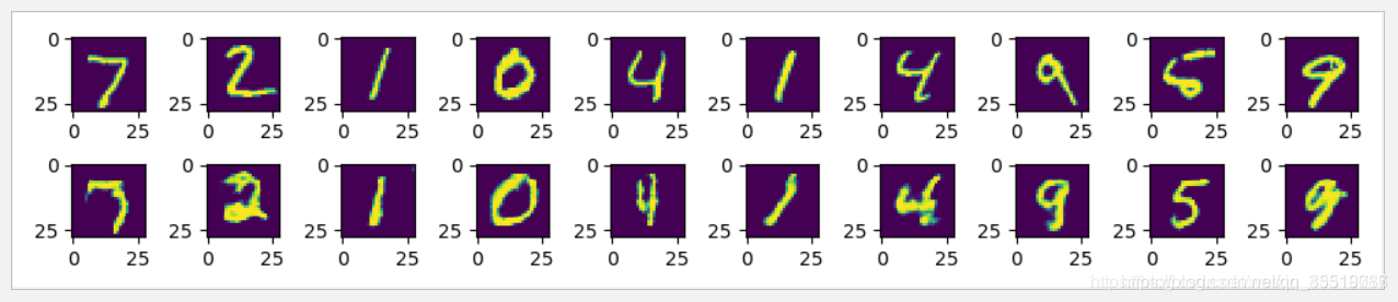
在12-4基础上,使用GAN-cls技术对判别器进行改造,并通过输入错误的样本标签让判别器学习样本与标签的匹配,从而优化生成器,使生成器最终生成与标签一直的样本,实现与ACGAN等同的效果。
程序:
import numpy as np
import tensorflow as tf
import matplotlib.pyplot as plt
from scipy.stats import norm
import tensorflow.contrib.slim as slim

from tensorflow.examples.tutorials.mnist import input_data

mnist = input_data.read_data_sets("/data/")  # , one_hot=True)

tf.reset_default_graph()


def generator(x):
    reuse = len([t for t in tf.global_variables() if t.name.startswith('generator')]) > 0
    with tf.variable_scope('generator', reuse=reuse):
        # 两个全连接
        x = slim.fully_connected(x, 1024)
        x = slim.batch_norm(x, activation_fn=tf.nn.relu)
        x = slim.fully_connected(x, 7 * 7 * 128)
        x = slim.batch_norm(x, activation_fn=tf.nn.relu)
        x = tf.reshape(x, [-1, 7, 7, 128])
        # 两个转置卷积
        x = slim.conv2d_transpose(x, 64, kernel_size=[4, 4], stride=2, activation_fn=None)
        x = slim.batch_norm(x, activation_fn=tf.nn.relu)
        z = slim.conv2d_transpose(x, 1, kernel_size=[4, 4], stride=2, activation_fn=tf.nn.sigmoid)
    return z


def leaky_relu(x):
    return tf.where(tf.greater(x, 0), x, 0.01 * x)


batch_size = 10  # 最小批次
classes_dim = 10  # 10 个分类

rand_dim = 38
n_input = 784
'''------------------------------------------------'''
#1 修改判别器

def discriminator(x, y):
    reuse = len([t for t in tf.global_variables() if t.name.startswith('discriminator')]) > 0
    with tf.variable_scope('discriminator', reuse=reuse):
        y = slim.fully_connected(y, num_outputs=n_input, activation_fn=leaky_relu)
        y = tf.reshape(y, shape=[-1, 28, 28, 1])
        x = tf.reshape(x, shape=[-1, 28, 28, 1])

        x = tf.concat(axis=3, values=[x, y])
        x = slim.conv2d(x, num_outputs=64, kernel_size=[4, 4], stride=2, activation_fn=leaky_relu)
        x = slim.conv2d(x, num_outputs=128, kernel_size=[4, 4], stride=2, activation_fn=leaky_relu)
        x = slim.flatten(x)
        shared_tensor = slim.fully_connected(x, num_outputs=1024, activation_fn=leaky_relu)
        disc = slim.fully_connected(shared_tensor, num_outputs=1, activation_fn=tf.nn.sigmoid)
        disc = tf.squeeze(disc, -1)

    return disc
'''------------------------------------------------'''
#2 添加错误标签输入符

x = tf.placeholder(tf.float32, [None, n_input])#输入样本
y = tf.placeholder(tf.int32, [None])#正确标签
misy = tf.placeholder(tf.int32, [None])#错误标签

z_rand = tf.random_normal((batch_size, rand_dim))  # 38列
z = tf.concat(axis=1, values=[tf.one_hot(y, depth=classes_dim), z_rand])  # 50列
gen = generator(z)
genout = tf.squeeze(gen, -1)

# 判别器
xin = tf.concat([x, tf.reshape(gen, shape=[-1, 784]), x], 0)
yin = tf.concat(
    [tf.one_hot(y, depth=classes_dim), tf.one_hot(y, depth=classes_dim), tf.one_hot(misy, depth=classes_dim)], 0)
disc_all = discriminator(xin, yin)
disc_real, disc_fake, disc_mis = tf.split(disc_all, 3)

loss_d = tf.reduce_sum(tf.square(disc_real - 1) + (tf.square(disc_fake) + tf.square(disc_mis)) / 2) / 2
loss_g = tf.reduce_sum(tf.square(disc_fake - 1)) / 2
'''------------------------------------------------'''

# 获得各个网络中各自的训练参数
t_vars = tf.trainable_variables()
d_vars = [var for var in t_vars if 'discriminator' in var.name]
g_vars = [var for var in t_vars if 'generator' in var.name]

# disc_global_step = tf.Variable(0, trainable=False)
gen_global_step = tf.Variable(0, trainable=False)
'''------------------------------------------------'''
#3 使用MonitoredTrainingSession创建session,开始训练

global_step = tf.train.get_or_create_global_step()  # 使用MonitoredTrainingSession,必须有

train_disc = tf.train.AdamOptimizer(0.0001).minimize(loss_d, var_list=d_vars, global_step=global_step)
train_gen = tf.train.AdamOptimizer(0.001).minimize(loss_g, var_list=g_vars, global_step=gen_global_step)

training_epochs = 3
display_step = 1

with tf.train.MonitoredTrainingSession(checkpoint_dir='log/checkpointsnew', save_checkpoint_secs=60) as sess:
    total_batch = int(mnist.train.num_examples / batch_size)
    print("global_step.eval(session=sess)", global_step.eval(session=sess),
          int(global_step.eval(session=sess) / total_batch))
    for epoch in range(int(global_step.eval(session=sess) / total_batch), training_epochs):
        avg_cost = 0.

        # 遍历全部数据集
        for i in range(total_batch):
            batch_xs, batch_ys = mnist.train.next_batch(batch_size)  # 取数据
            _, mis_batch_ys = mnist.train.next_batch(batch_size)  # 取数据
            feeds = {x: batch_xs, y: batch_ys, misy: mis_batch_ys}

            # Fit training using batch data
            l_disc, _, l_d_step = sess.run([loss_d, train_disc, global_step], feeds)
            l_gen, _, l_g_step = sess.run([loss_g, train_gen, gen_global_step], feeds)
            '''--------------------------------------------------------------------'''

        # 显示训练中的详细信息
        if epoch % display_step == 0:
            print("Epoch:", '%04d' % (epoch + 1), "cost=", "{:.9f} ".format(l_disc), l_gen)

    print("完成!")

    # 测试
    _, mis_batch_ys = mnist.train.next_batch(batch_size)
    print("result:",
          loss_d.eval({x: mnist.test.images[:batch_size], y: mnist.test.labels[:batch_size], misy: mis_batch_ys},
                      session=sess)
          , loss_g.eval({x: mnist.test.images[:batch_size], y: mnist.test.labels[:batch_size], misy: mis_batch_ys},
                        session=sess))

    # 根据图片模拟生成图片
    show_num = 10
    gensimple, inputx, inputy = sess.run(
        [genout, x, y], feed_dict={x: mnist.test.images[:batch_size], y: mnist.test.labels[:batch_size]})

    f, a = plt.subplots(2, 10, figsize=(10, 2))
    for i in range(show_num):
        a[0][i].imshow(np.reshape(inputx[i], (28, 28)))
        a[1][i].imshow(np.reshape(gensimple[i], (28, 28)))

    plt.draw()
    plt.show()
结果:
…
global_step.eval(session=sess) 0 0
Epoch: 0001 cost= 0.690422952  4.9999237
Epoch: 0002 cost= 1.249726415  2.4782877
Epoch: 0003 cost= 1.146144152  1.6790285
完成!
result: 1.3178995 1.5426748
GAN-cls结果:
12.6 mnistEspcn
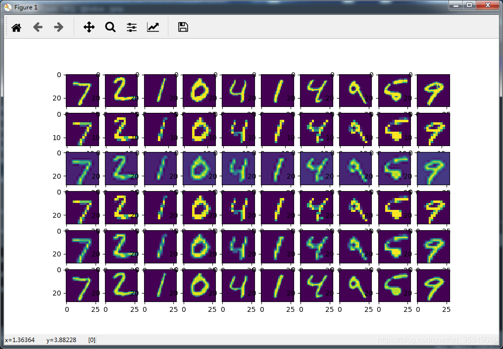
ESPCN实现MNIST数据集的超分辨率重建
程序:
import tensorflow as tf
import matplotlib.pyplot as plt
import numpy as np
import tensorflow.contrib.slim as slim
from tensorflow.examples.tutorials.mnist import input_data

mnist = input_data.read_data_sets("/data/", one_hot=True)

# print(__author__)

batch_size = 30  # 获取样本的批次大小
n_input = 784  # MNIST data 输入 (img shape: 28*28)
n_classes = 10  # MNIST 列别 (0-9 ,一共10类)

# 待输入的样本图片
x = tf.placeholder("float", [None, n_input])
# x = mnist.train.image
img = tf.reshape(x, [-1, 28, 28, 1])
# corrupted image
x_small = tf.image.resize_bicubic(img, (14, 14))  # 缩小2倍

x_bicubic = tf.image.resize_bicubic(x_small, (28, 28))  # 双立方插值算法变化
x_nearest = tf.image.resize_nearest_neighbor(x_small, (28, 28))
x_bilin = tf.image.resize_bilinear(x_small, (28, 28))

# espcn
net = slim.conv2d(x_small, 64, 5)
net = slim.conv2d(net, 32, 3)
net = slim.conv2d(net, 4, 3)
net = tf.depth_to_space(net, 2)
print("net.shape", net.shape)

y_pred = tf.reshape(net, [-1, 784])

cost = tf.reduce_mean(tf.pow(x - y_pred, 2))
optimizer = tf.train.AdamOptimizer(0.01).minimize(cost)

training_epochs = 100
display_step = 20

with tf.Session() as sess:
    sess.run(tf.global_variables_initializer())
    total_batch = int(mnist.train.num_examples / batch_size)
    # 启动循环开始训练
    for epoch in range(training_epochs):
        # 遍历全部数据集
        for i in range(total_batch):
            batch_xs, batch_ys = mnist.train.next_batch(batch_size)
            _, c = sess.run([optimizer, cost], feed_dict={x: batch_xs})
        # 显示训练中的详细信息
        if epoch % display_step == 0:
            print("Epoch:", '%04d' % (epoch + 1),
                  "cost=", "{:.9f}".format(c))

    print("完成!")

    show_num = 10
    encode_s, encode_b, encode_n, encode_bi, y_predv = sess.run(
        [x_small, x_bicubic, x_nearest, x_bilin, y_pred], feed_dict={x: mnist.test.images[:show_num]})

    f, a = plt.subplots(6, 10, figsize=(10, 6))
    for i in range(show_num):
        a[0][i].imshow(np.reshape(mnist.test.images[i], (28, 28)))
        a[1][i].imshow(np.reshape(encode_s[i], (14, 14)))
        a[2][i].imshow(np.reshape(encode_b[i], (28, 28)))
        a[3][i].imshow(np.reshape(encode_n[i], (28, 28)))
        a[4][i].imshow(np.reshape(encode_bi[i], (28, 28)))
        a[5][i].imshow(np.reshape(y_predv[i], (28, 28)))
    plt.show()
结果:
Epoch: 0001 cost= 0.005226622
Epoch: 0021 cost= 0.004032122
Epoch: 0041 cost= 0.004496219
Epoch: 0061 cost= 0.004120507
Epoch: 0081 cost= 0.004602988
完成!
12-7 tfrecoderSRESPCN
通过使用ESPCN网络,在flower数据集上将低分辨率图片复原成高分辨率图片并与其他复原函数生成的结果进行比较。
程序:
#1 引入头文件,创建样本数据源
import tensorflow as tf
from slim.datasets import flowers
import numpy as np
import matplotlib.pyplot as plt

slim = tf.contrib.slim
'''----------------------------------------------'''
#6 构建图片质量评估函数

def batch_mse_psnr(dbatch):
    im1, im2 = np.split(dbatch, 2)
    mse = ((im1 - im2) ** 2).mean(axis=(1, 2))
    psnr = np.mean(20 * np.log10(255.0 / np.sqrt(mse)))
    return np.mean(mse), psnr


def batch_y_psnr(dbatch):
    r, g, b = np.split(dbatch, 3, axis=3)
    y = np.squeeze(0.3 * r + 0.59 * g + 0.11 * b)
    im1, im2 = np.split(y, 2)
    mse = ((im1 - im2) ** 2).mean(axis=(1, 2))
    psnr = np.mean(20 * np.log10(255.0 / np.sqrt(mse)))
    return psnr


def batch_ssim(dbatch):
    im1, im2 = np.split(dbatch, 2)
    imgsize = im1.shape[1] * im1.shape[2]
    avg1 = im1.mean((1, 2), keepdims=1)
    avg2 = im2.mean((1, 2), keepdims=1)
    std1 = im1.std((1, 2), ddof=1)
    std2 = im2.std((1, 2), ddof=1)
    cov = ((im1 - avg1) * (im2 - avg2)).mean((1, 2)) * imgsize / (imgsize - 1)
    avg1 = np.squeeze(avg1)
    avg2 = np.squeeze(avg2)
    k1 = 0.01
    k2 = 0.03
    c1 = (k1 * 255) ** 2
    c2 = (k2 * 255) ** 2
    c3 = c2 / 2
    return np.mean(
        (2 * avg1 * avg2 + c1) * 2 * (cov + c3) / (avg1 ** 2 + avg2 ** 2 + c1) / (std1 ** 2 + std2 ** 2 + c2))
'''----------------------------------------------'''

def showresult(subplot, title, orgimg, thisimg, dopsnr=True):
    p = plt.subplot(subplot)
    p.axis('off')
    p.imshow(np.asarray(thisimg[0], dtype='uint8'))
    if dopsnr:
        conimg = np.concatenate((orgimg, thisimg))
        mse, psnr = batch_mse_psnr(conimg)
        ypsnr = batch_y_psnr(conimg)
        ssim = batch_ssim(conimg)
        p.set_title(title + str(int(psnr)) + " y:" + str(int(ypsnr)) + " s:" + str(ssim))
    else:
        p.set_title(title)


height = width = 200
batch_size = 4
DATA_DIR = "D:/tmp/data/flowers"

# 选择数据集validation
dataset = flowers.get_split('validation', DATA_DIR)
# 创建一个provider
provider = slim.dataset_data_provider.DatasetDataProvider(dataset, num_readers=2)
# 通过provider的get拿到内容
[image, label] = provider.get(['image', 'label'])
print(image.shape)
'''----------------------------------------------'''
#2 获取批次样本并通过TensorFlow函数实现超分辨率

# 剪辑图片为统一大小
distorted_image = tf.image.resize_image_with_crop_or_pad(image, height, width)  # 剪辑尺寸,不够填充
################################################
images, labels = tf.train.batch([distorted_image, label], batch_size=batch_size)
print(images.shape)

x_smalls = tf.image.resize_images(images, (np.int32(height / 2), np.int32(width / 2)))  # 缩小2*2倍
x_smalls2 = x_smalls / 255.0
# 还原
x_nearests = tf.image.resize_images(x_smalls, (height, width), tf.image.ResizeMethod.NEAREST_NEIGHBOR)
x_bilins = tf.image.resize_images(x_smalls, (height, width), tf.image.ResizeMethod.BILINEAR)
x_bicubics = tf.image.resize_images(x_smalls, (height, width), tf.image.ResizeMethod.BICUBIC)
'''----------------------------------------------'''
#3 建立ESPCN网络结构

net = slim.conv2d(x_smalls2, 64, 5, activation_fn=tf.nn.tanh)
net = slim.conv2d(net, 32, 3, activation_fn=tf.nn.tanh)
net = slim.conv2d(net, 12, 3, activation_fn=None)  # 2*2*3
y_predt = tf.depth_to_space(net, 2)

y_pred = y_predt * 255.0
y_pred = tf.maximum(y_pred, 0)
y_pred = tf.minimum(y_pred, 255)

dbatch = tf.concat([tf.cast(images, tf.float32), y_pred], 0)
'''----------------------------------------------'''
#4 构建loss及优化器

cost = tf.reduce_mean(tf.pow(tf.cast(images, tf.float32) / 255.0 - y_predt, 2))
optimizer = tf.train.AdamOptimizer(0.000001).minimize(cost)
'''----------------------------------------------'''
#5 建立session,运行

training_epochs = 150000
display_step = 200

sess = tf.InteractiveSession()
sess.run(tf.global_variables_initializer())

# 启动队列
tf.train.start_queue_runners(sess=sess)

# 启动循环开始训练
for epoch in range(training_epochs):

    _, c = sess.run([optimizer, cost])

    # 显示训练中的详细信息
    if epoch % display_step == 0:
        d_batch = dbatch.eval()
        mse, psnr = batch_mse_psnr(d_batch)
        ypsnr = batch_y_psnr(d_batch)
        ssim = batch_ssim(d_batch)
        print("Epoch:", '%04d' % (epoch + 1),
              "cost=", "{:.9f}".format(c), "psnr", psnr, "ypsnr", ypsnr, "ssim", ssim)

print("完成!")
'''----------------------------------------------'''
#7 图示结果

imagesv, label_batch, x_smallv, x_nearestv, x_bilinv, x_bicubicv, y_predv = sess.run(
    [images, labels, x_smalls, x_nearests, x_bilins, x_bicubics, y_pred])
print("原", np.shape(imagesv), "缩放后的", np.shape(x_smallv), label_batch)

###显示
plt.figure(figsize=(20, 10))

showresult(161, "org", imagesv, imagesv, False)
showresult(162, "small/4", imagesv, x_smallv, False)
showresult(163, "near", imagesv, x_nearestv)
showresult(164, "biline", imagesv, x_bilinv)
showresult(165, "bicubicv", imagesv, x_bicubicv)
showresult(166, "pred", imagesv, y_predv)

plt.show()

#
## 可视化结果
# plt.figure(figsize=(20,10))
# p1 = plt.subplot(161)
# p2 = plt.subplot(162)
# p3 = plt.subplot(163)
# p4 = plt.subplot(164)
# p5 = plt.subplot(165)
# p6 = plt.subplot(166)
# p1.axis('off')
# p2.axis('off')
# p3.axis('off')
# p4.axis('off')
# p5.axis('off')
# p6.axis('off')
#
#
# p1.imshow(imagesv[0])# 显示图片
# p2.imshow(np.asarray(x_smallv[0], dtype='uint8') )# 显示图片,必须转成uint8才能打印出来
# p3.imshow(np.asarray(x_nearestv[0], dtype='uint8')  )# 显示图片
# p4.imshow(np.asarray(x_bilinv[0], dtype='uint8') )# 显示图片
# p5.imshow(np.asarray(x_bicubicv[0], dtype='uint8') )# 显示图片
# p6.imshow(np.asarray(y_predv[0], dtype='uint8') )# 显示图片
#
# p1.set_title("org")
# p2.set_title("small/4")
# p3.set_title("near")
# p4.set_title("biline")
# p5.set_title("bicubicv")
# p6.set_title("pred")
# plt.show()
结果:
(?, ?, 3)
(4, 200, 200, 3)
Epoch: 0001 cost= 0.360416085 psnr 6.669006 ypsnr 6.8186326 ssim 0.021616353
Epoch: 0201 cost= 0.331164747 psnr 8.1468115 ypsnr 7.0099936 ssim 0.030560756
Epoch: 0401 cost= 0.298657089 psnr 6.903029 ypsnr 6.9319057 ssim 0.03709429
Epoch: 0601 cost= 0.278883010 psnr 8.724986 ypsnr 8.624394 ssim 0.0352783
Epoch: 0801 cost= 0.266729325 psnr 6.616158 ypsnr 6.7454033 ssim 0.052763406
Epoch: 1001 cost= 0.221033752 psnr 8.113207 ypsnr 8.400061 ssim 0.08303006
Epoch: 1201 cost= 0.248143092 psnr 8.751854 ypsnr 8.84062 ssim 0.13017127
Epoch: 1401 cost= 0.243928418 psnr 9.626335 ypsnr 10.030566 ssim 0.15815271
Epoch: 1601 cost= 0.190259323 psnr 8.577847 ypsnr 9.032168 ssim 0.14702274
Epoch: 1801 cost= 0.157699853 psnr 11.350587 ypsnr 11.985262 ssim 0.2490645
Epoch: 2001 cost= 0.123353019 psnr 9.742246 ypsnr 10.396275 ssim 0.20674324
Epoch: 2201 cost= 0.115382612 psnr 8.905223 ypsnr 9.6788645 ssim 0.24067946
......
Epoch: 148001 cost= 0.002764479 psnr 26.83477 ypsnr 26.944088 ssim 0.9765523
Epoch: 148201 cost= 0.005125942 psnr 24.819565 ypsnr 25.221066 ssim 0.92076725
Epoch: 148401 cost= 0.002659404 psnr 28.065817 ypsnr 28.351946 ssim 0.9765806
Epoch: 148601 cost= 0.002774108 psnr 24.86807 ypsnr 26.140589 ssim 0.9535808
Epoch: 148801 cost= 0.002453615 psnr 27.56114 ypsnr 27.631792 ssim 0.97236115
Epoch: 149001 cost= 0.004432773 psnr 25.963507 ypsnr 26.101135 ssim 0.9683759
Epoch: 149201 cost= 0.002581447 psnr 27.878935 ypsnr 28.195324 ssim 0.9630526
Epoch: 149401 cost= 0.004874272 psnr 26.993256 ypsnr 27.916882 ssim 0.97514504
Epoch: 149601 cost= 0.002618119 psnr 26.826574 ypsnr 26.896557 ssim 0.91461986
Epoch: 149801 cost= 0.003381842 psnr 23.671938 ypsnr 24.175095 ssim 0.90275687
完成!
原 (4, 200, 200, 3) 缩放后的 (4, 100, 100, 3) [4 2 3 3]
ESPCN实例flowers结果:

12-8 resESPCN
将flower数据集中的图片转换成低分辨率,再通过使用带残差网络的ESPCN网络复原成高分辨率图片,并与其他复原函数的生成结果进行比较。
程序:
import tensorflow as tf
from slim.datasets import flowers
import numpy as np
import matplotlib.pyplot as plt
import os

slim = tf.contrib.slim

tf.reset_default_graph()


def batch_mse_psnr(dbatch):
    im1, im2 = np.split(dbatch, 2)
    mse = ((im1 - im2) ** 2).mean(axis=(1, 2))
    psnr = np.mean(20 * np.log10(255.0 / np.sqrt(mse)))
    return np.mean(mse), psnr


def batch_y_psnr(dbatch):
    r, g, b = np.split(dbatch, 3, axis=3)
    y = np.squeeze(0.3 * r + 0.59 * g + 0.11 * b)
    im1, im2 = np.split(y, 2)
    mse = ((im1 - im2) ** 2).mean(axis=(1, 2))
    psnr = np.mean(20 * np.log10(255.0 / np.sqrt(mse)))
    return psnr


def batch_ssim(dbatch):
    im1, im2 = np.split(dbatch, 2)
    imgsize = im1.shape[1] * im1.shape[2]
    avg1 = im1.mean((1, 2), keepdims=1)
    avg2 = im2.mean((1, 2), keepdims=1)
    std1 = im1.std((1, 2), ddof=1)
    std2 = im2.std((1, 2), ddof=1)
    cov = ((im1 - avg1) * (im2 - avg2)).mean((1, 2)) * imgsize / (imgsize - 1)
    avg1 = np.squeeze(avg1)
    avg2 = np.squeeze(avg2)
    k1 = 0.01
    k2 = 0.03
    c1 = (k1 * 255) ** 2
    c2 = (k2 * 255) ** 2
    c3 = c2 / 2
    return np.mean(
        (2 * avg1 * avg2 + c1) * 2 * (cov + c3) / (avg1 ** 2 + avg2 ** 2 + c1) / (std1 ** 2 + std2 ** 2 + c2))


def showresult(subplot, title, orgimg, thisimg, dopsnr=True):
    p = plt.subplot(subplot)
    p.axis('off')
    p.imshow(np.asarray(thisimg[0], dtype='uint8'))
    if dopsnr:
        conimg = np.concatenate((orgimg, thisimg))
        mse, psnr = batch_mse_psnr(conimg)
        ypsnr = batch_y_psnr(conimg)
        ssim = batch_ssim(conimg)
        p.set_title(title + str(int(psnr)) + " y:" + str(int(ypsnr)) + " s:" + " s:%.4f" % ssim)
    else:
        p.set_title(title)


height = width = 256
batch_size = 16
DATA_DIR = "D:/tmp/data/flowers"

# 选择数据集validation
dataset = flowers.get_split('validation', DATA_DIR)
# 创建一个provider
provider = slim.dataset_data_provider.DatasetDataProvider(dataset, num_readers=2)
# 通过provider的get拿到内容
[image, label] = provider.get(['image', 'label'])
print(image.shape)

# 剪辑图片为统一大小
distorted_image = tf.image.resize_image_with_crop_or_pad(image, height, width)  # 剪辑尺寸,不够填充
################################################
'''----------------------------------------------'''
#1 修改输入图片分辨率
images, labels = tf.train.batch([distorted_image, label], batch_size=batch_size)
print(images.shape)

x_smalls = tf.image.resize_images(images, (np.int32(height / 4), np.int32(width / 4)))  # 缩小4*4倍
x_smalls2 = x_smalls / 255.0
'''----------------------------------------------'''

# 还原
x_nearests = tf.image.resize_images(x_smalls, (height, width), tf.image.ResizeMethod.NEAREST_NEIGHBOR)
x_bilins = tf.image.resize_images(x_smalls, (height, width), tf.image.ResizeMethod.BILINEAR)
x_bicubics = tf.image.resize_images(x_smalls, (height, width), tf.image.ResizeMethod.BICUBIC)


####################################
# net = slim.conv2d(x_smalls2, 64, 5,activation_fn = tf.nn.tanh)
# net =slim.conv2d(net, 256, 3,activation_fn = tf.nn.tanh)
# net = tf.depth_to_space(net,2) #64
# net =slim.conv2d(net, 64, 3,activation_fn = tf.nn.tanh)
# net = tf.depth_to_space(net,2) #16
# y_predt = slim.conv2d(net, 3, 3,activation_fn = None)#2*2*3

######################################
'''----------------------------------------------'''
#2 添加残差网络

def leaky_relu(x, alpha=0.1, name='lrelu'):
    with tf.name_scope(name):
        x = tf.maximum(x, alpha * x)
        return x


def residual_block(nn, i, name='resblock'):
    with tf.variable_scope(name + str(i)):
        conv1 = slim.conv2d(nn, 64, 3, activation_fn=leaky_relu, normalizer_fn=slim.batch_norm)
        conv2 = slim.conv2d(conv1, 64, 3, activation_fn=leaky_relu, normalizer_fn=slim.batch_norm)
        return tf.add(nn, conv2)

net = slim.conv2d(x_smalls2, 64, 5, activation_fn=leaky_relu)
block = []
for i in range(16):
    block.append(residual_block(block[-1] if i else net, i))
conv2 = slim.conv2d(block[-1], 64, 3, activation_fn=leaky_relu, normalizer_fn=slim.batch_norm)
sum1 = tf.add(conv2, net)

conv3 = slim.conv2d(sum1, 256, 3, activation_fn=None)
ps1 = tf.depth_to_space(conv3, 2)
relu2 = leaky_relu(ps1)
conv4 = slim.conv2d(relu2, 256, 3, activation_fn=None)
ps2 = tf.depth_to_space(conv4, 2)  # 再放大两倍 64
relu3 = leaky_relu(ps2)
y_predt = slim.conv2d(relu3, 3, 3, activation_fn=None)  # 输出
'''----------------------------------------------'''

y_pred = y_predt * 255.0
y_pred = tf.maximum(y_pred, 0)
y_pred = tf.minimum(y_pred, 255)

dbatch = tf.concat([tf.cast(images, tf.float32), y_pred], 0)
'''----------------------------------------------'''
#3 修改学习率,进行网络训练

learn_rate = 0.001

cost = tf.reduce_mean(tf.pow(tf.cast(images, tf.float32) / 255.0 - y_predt, 2))
optimizer = tf.train.AdamOptimizer(learn_rate).minimize(cost)
# training_epochs =100000
# display_step =5000

training_epochs = 10000
'''----------------------------------------------'''

display_step = 400
'''----------------------------------------------'''
#4 添加检查点

flags = 'b' + str(batch_size) + '_h' + str(height / 4) + '_r' + str(
    learn_rate) + '_res'  # set for practicers to try different setups
# flags='b'+str(batch_size)+'_r'+str(height/4)+'_depth_conv2d'#set for practicers to try different setups
if not os.path.exists('save'):
    os.mkdir('save')
save_path = 'save/tf_' + flags
if not os.path.exists(save_path):
    os.mkdir(save_path)
saver = tf.train.Saver(max_to_keep=1)  # 生成saver

sess = tf.InteractiveSession()
sess.run(tf.global_variables_initializer())

kpt = tf.train.latest_checkpoint(save_path)
print(kpt)
startepo = 0
if kpt != None:
    saver.restore(sess, kpt)
    ind = kpt.find("-")
    startepo = int(kpt[ind + 1:])
    print("startepo=", startepo)

# 启动队列
tf.train.start_queue_runners(sess=sess)

# 启动循环开始训练
for epoch in range(startepo, training_epochs):

    _, c = sess.run([optimizer, cost])

    # 显示训练中的详细信息
    if epoch % display_step == 0:
        d_batch = dbatch.eval()
        mse, psnr = batch_mse_psnr(d_batch)
        ypsnr = batch_y_psnr(d_batch)
        ssim = batch_ssim(d_batch)
        print("Epoch:", '%04d' % (epoch + 1),
              "cost=", "{:.9f}".format(c), "psnr", psnr, "ypsnr", ypsnr, "ssim", ssim)

        saver.save(sess, save_path + "/tfrecord.cpkt", global_step=epoch)
print("完成!")
saver.save(sess, save_path + "/tfrecord.cpkt", global_step=epoch)
'''----------------------------------------------'''

imagesv, label_batch, x_smallv, x_nearestv, x_bilinv, x_bicubicv, y_predv = sess.run(
    [images, labels, x_smalls, x_nearests, x_bilins, x_bicubics, y_pred])
print("原", np.shape(imagesv), "缩放后的", np.shape(x_smallv), label_batch)

#        print(np.max(imagesv[0]),np.max(x_bilinv[0]),np.max(x_bicubicv[0]),np.max(y_predv[0]))
#        print(np.min(imagesv[0]),np.min(x_bilinv[0]),np.min(x_bicubicv[0]),np.min(y_predv[0]))

###显示
plt.figure(figsize=(20, 10))

showresult(161, "org", imagesv, imagesv, False)
showresult(162, "small/4", imagesv, x_smallv, False)
showresult(163, "near", imagesv, x_nearestv)
showresult(164, "biline", imagesv, x_bilinv)
showresult(165, "bicubicv", imagesv, x_bicubicv)
showresult(166, "pred", imagesv, y_predv)

plt.show()
结果:
(?, ?, 3)
(16, 256, 256, 3)
None

Epoch: 0001 cost= 0.211108640 psnr 11.407981 ypsnr 13.488435 ssim 0.3307791485562411
Epoch: 0401 cost= 0.011509083 psnr 21.501999 ypsnr 21.893381 ssim 0.9146646896505927
Epoch: 0801 cost= 0.006142357 psnr 22.968485 ypsnr 23.852066 ssim 0.9279918317009753
Epoch: 1201 cost= 0.005762197 psnr 23.517471 ypsnr 23.978153 ssim 0.9582196990382146
Epoch: 1601 cost= 0.005582960 psnr 21.631796 ypsnr 21.95909 ssim 0.9040559790367432
Epoch: 2001 cost= 0.006873480 psnr 22.270742 ypsnr 22.955856 ssim 0.9182121559303617
Epoch: 2401 cost= 0.005612638 psnr 22.760986 ypsnr 23.089485 ssim 0.9262228042835311
Epoch: 2801 cost= 0.005443098 psnr 23.420565 ypsnr 23.99352 ssim 0.9442156526190871
Epoch: 3201 cost= 0.005806287 psnr 23.749552 ypsnr 24.477228 ssim 0.9450137807004954
Epoch: 3601 cost= 0.005395472 psnr 25.262682 ypsnr 25.838692 ssim 0.9542044947249698
Epoch: 4001 cost= 0.006084155 psnr 22.919348 ypsnr 23.530197 ssim 0.9359309824799281
Epoch: 4401 cost= 0.005560590 psnr 25.203331 ypsnr 25.738913 ssim 0.9530244535767078
Epoch: 4801 cost= 0.004648690 psnr 25.333511 ypsnr 25.992489 ssim 0.9402358180894312
Epoch: 5201 cost= 0.003865756 psnr 25.506927 ypsnr 25.824717 ssim 0.9539453031428664
Epoch: 5601 cost= 0.003216719 psnr 24.912142 ypsnr 25.47681 ssim 0.9475247548633271
Epoch: 6001 cost= 0.004854371 psnr 23.78054 ypsnr 24.404945 ssim 0.9592952459358722
Epoch: 6401 cost= 0.003208177 psnr 26.982233 ypsnr 27.602211 ssim 0.974860297423353
Epoch: 6801 cost= 0.004153049 psnr 24.687653 ypsnr 25.168243 ssim 0.94472342376237
Epoch: 7201 cost= 0.004355598 psnr 27.507273 ypsnr 28.3989 ssim 0.9794754731337089
Epoch: 7601 cost= 0.006875461 psnr 24.117432 ypsnr 24.569798 ssim 0.9477540112962018
Epoch: 8001 cost= 0.006706636 psnr 22.219862 ypsnr 22.79896 ssim 0.9211242007323356
Epoch: 8401 cost= 0.004559200 psnr 24.15137 ypsnr 24.684011 ssim 0.9578859948346384
Epoch: 8801 cost= 0.005599694 psnr 24.537134 ypsnr 25.12828 ssim 0.9583166929362248
Epoch: 9201 cost= 0.005546704 psnr 23.239655 ypsnr 23.372845 ssim 0.9045935260983738
Epoch: 9601 cost= 0.006495696 psnr 24.761713 ypsnr 25.204636 ssim 0.953236243712651
完成!
原 (16, 256, 256, 3) 缩放后的 (16, 64, 64, 3) [3 3 0 4 4 2 3 0 3 4 3 3 0 2 3 2]


 6353


 扫一扫


 被折叠的 条评论
为什么被折叠?
 到【灌水乐园】发言


