线性逻辑回归的梯度下降算法python实现

线性逻辑回归的梯度下降算法python实现

前言： 逻辑回归是解决分类问题的一种的方法，关于逻辑回归的具体理论知识请至我的博文中查看

一、逻辑回归python实现示例代码

import matplotlib.pyplot as plt
import numpy as np
from sklearn.metrics import classification_report
from sklearn import preprocessing

# 数据是否需要标准化
scale = False
# 读取数据
data = np.genfromtxt('LR-testSet.csv', delimiter=',')
x_data = data[:, 0:-1]
y_data = data[:, -1, np.newaxis]

# 绘制各类别的数据散点图
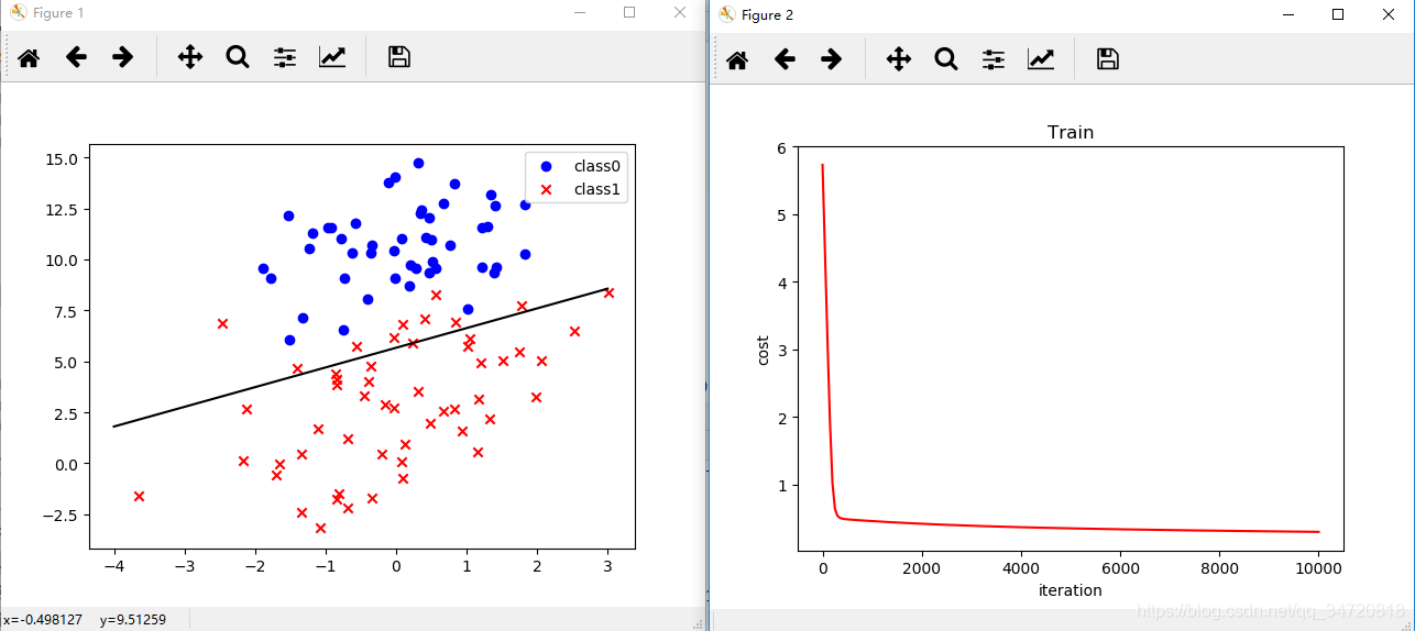
def plotClass():
    x0 = []
    y0 = []
    x1 = []
    y1 = []
    for i in range(len(x_data)):
        if y_data[i] == 0:
            x0.append(x_data[i, 0])
            y0.append(x_data[i, 1])
        else:
            x1.append(x_data[i, 0])
            y1.append(x_data[i, 1])

    # 绘图
    s1 = plt.scatter(x0, y0, c='b', marker='o')
    s2 = plt.scatter(x1, y1, c='r', marker='x')
    plt.legend(handles=[s1, s2], labels=['class0', 'class1'])


# 给样本添加偏置值项
X_data = np.concatenate((np.ones((100, 1)), x_data), axis=1)


# 定义逻辑回归的模型函数（S型函数）
def sigmoid(x):
    return 1 / (1 + np.exp(-x))


# 计算代价值
def cost(xMat, yMat, ws):
    left = np.multiply(yMat, np.log(sigmoid(xMat * ws)))
    right = np.multiply(1 - yMat, np.log(1 - sigmoid(xMat * ws)))
    return np.sum(left + right) / -len(xMat)


# 梯度下降算法
def gradAscent(xArr, yArr):
    if scale:
        xArr = preprocessing.scale(xArr)
    xMat = np.mat(xArr)
    yMat = np.mat(yArr)

    # 学习率
    lr = 0.001
    # 梯度下降迭代次数
    ite = 10000
    # 记录梯度下降过程中的代价值
    costList = []
    # 计算数据行列数
    m, n = np.shape(xMat)
    # 初始化线性函数权重
    ws = np.mat(np.ones((n, 1)))
    for i in range(ite + 1):
        h = sigmoid(xMat * ws)
        ws_grad = xMat.T * (h - yMat) / m
        ws = ws - lr * ws_grad
        if i % 50 == 0:
            costList.append(cost(xMat, yMat, ws))
    return ws, costList
ws, costList = gradAscent(X_data, y_data)
# 画决策边界
if not scale:
    plotClass()
    x_test = [[-4], [3]]
    y_test = (-ws[0] - x_test * ws[1]) / ws[2]
    plt.plot(x_test, y_test, 'k')

# 绘制代价值的变化
plt.figure()
x = np.linspace(0, 10000, 201)
plt.plot(x, costList, c='r')
plt.title('Train')
plt.xlabel('iteration')
plt.ylabel('cost')

# 根据训练的模型进行预测类型
def predict(x_data, ws):
    if scale:
        x_data = preprocessing.scale(x_data)
    xMat = np.mat(x_data)
    ws = np.mat(ws)
    return [1 if x >= 0.5 else 0 for x in sigmoid(xMat * ws)]

predictions = predict(X_data, ws)
# 计算准确率，召回率，F1值
print(classification_report(y_data, predictions))
plt.show()

二、执行结果

              precision    recall  f1-score   support

         0.0       0.82      1.00      0.90        47
         1.0       1.00      0.81      0.90        53

   micro avg       0.90      0.90      0.90       100
   macro avg       0.91      0.91      0.90       100
weighted avg       0.92      0.90      0.90       100

三、数据下载
链接：https://pan.baidu.com/s/1cOxjGUyVbf3qDtPFPJKqwA
提取码：1mlo