用Maple解决曲线绕轴旋转成面问题

最新推荐文章于 2024-03-26 19:30:53 发布

原创最新推荐文章于 2024-03-26 19:30:53 发布 · 1.9k 阅读

4 ·

CC 4.0 BY-SA版权

文章标签：

#Maple #曲线旋转

新年期间Maple技术交互研讨群发布如下题目以活跃群氛围：

此题本意是想让大家通过数据处理来实现最终旋转效果，因此几个参考命令都是围绕这一目的。但是，由于测试函数简单，最终没能把答者思路往这方面引导。这里，先给出群友“浮夸的货”的源程序：

z:=y^2;
k:=1;curve_point:=`<,>`(0,y,z);
foot_perpendicular:=`<,>`(0,(k*z+y)/(k^2+1),k*(k*z+y)/(k^2+1));
a:=curve_point-foot_perpendicular;
n1:=`<,>`(0,k/sqrt(k^2+1),-1/sqrt(k^2+1));
n2:=`<,>`(1,0,0);n3:=cos(tau)*n1+sin(tau)*n2;
rotate_point:=simplify(foot_perpendicular+n3*norm(a,2))

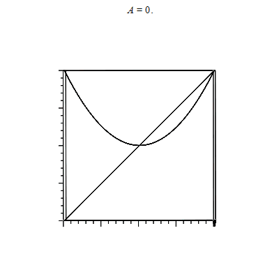
with(plots)：
display(animate(plot3d,[[sqrt(abs(k)^2+1)*sin(tau)*(k*y-z)/(k^2+1),(k*cos(tau)*sqrt(abs(k)^2+1)*(k^2+1)*((k*y-z)/(k^2+1))+(k*z+y)*sqrt(k^2+1))/(k^2+1)^(3/2),-(cos(tau)*sqrt(abs(k)^2+1)*(k^2+1)*((k*y-z)/(k^2+1))-k*sqrt(k^2+1)*(k*z+y))/(k^2+1)^(3/2)],y=-1..1,tau=0..2*A],A=0..Pi),plot3d([0,y,k*y],y=-1..1))

第一段是单点绕轴旋转得到旋转点集三维参数表达rotate_point。第二段直接用animate追加plot3d([坐标参数])然后画出效果如下

数据成图，集图成动图。动图也不过是一帧一帧叠加而成。如果仔细查看动图制作代码，是可以发现改进的地方：

这里A相当于旋转多少角度，将之生成离散序列。比如说，最终生成0°:12°:360°角度序列。我们会发现，24°角包含12°角所绘曲面，36°角包含12°，24°所绘曲面……以此类推，这里面存在很明显的数据冗余。实际上，如果能一开始吧整个面数据求出来，反而能规避掉这一点。

再者，本次测试函数是“朴实”的二次函数如此确实可行。但如果初始曲线很复杂呢？出题意图是在帮一位朋友作一次曲线绕轴旋转时产生的，这条2维曲线十分复杂(xy坐标无显式函数关系且各自是复杂函数的积分表达式。在已作运算简化的基础上，平均一条曲线需要2分钟)，如果采用上面作图思路，它会重复绘制数倍曲线，最终造成时空强烈消耗（旋转面无非是多条曲线生成，Maple 默认animate帧数是25，上述程序粗略估计消耗50分钟+）。

因此，我解决那个问题思路基础是，先利用命令getdata得到初始曲线离散点数据,再基于理论rotate_point参数表达式得到整个面离散点数据surfacedata，进而使用命令surfdata绘制指定旋转角度曲面，最终配合命令display(plot_arrays,insequence=true)制作动图。这样子，整个旋转作用的对象将会更加广泛，效果也会好。这里直接上两段代码并作简短讲解。由于出题目另一方面在于让答者更多体会Maple一些实用命令，所以部分看着low的笔法我也会特地强调甚至给出评价，希望看的朋友不要介意。

#Janesefor do it in 2019/2/2 22:00 with Maple2018~
filename:="C:/Users/ysl-pc/Desktop/":
curve_point,foot_perpendicular:=<0|y2d|z2d>,<0|(y2d+k*z2d)/(k^2+1)|k*(y2d+k*z2d)/(k^2+1)>;
fp_cp:=curve_point-foot_perpendicular;
n1,n2:=<0|k/sqrt(k^2+1)|-1/sqrt(k^2+1)>,<1|0|0>;
n_tau:=cos(tau)*n1+sin(tau)*n2;
rotate_point:=simplify(foot_perpendicular+n_tau*norm(fp_cp,2))assuming k>0;
rotate_point_down:=rotate_point;
rotate_point_up:=eval(rotate_point_down,tau=tau+Pi);
fastarray:=(tx,ty,tz)->zip((tx,ty)->[tx[],ty],zip(`[]`,tx,ty),tz);
location_adjust:=(t,temp_expr)->if t[1] then subs(t[2..3],temp_expr[1])
                    else subs(t[2..3],temp_expr[2]) end if;

save rotate_point_down,rotate_point_up,rotate_point,fastarray,location_adjust,cat(filename,"necassary_results.mw")

本次辅助结论、函数较多，写进一个文件显得“喧宾夺主”。因此特地在一个次要文件里面包含它们。这里文件地址我选的是桌面。特别强调：Windows系统下，Maple承认地址格式是带“/”而非"\"，因此复制地址后要进行调整。注意轴上轴下相差一个π相位，表达式有所区别，体会学习如何保存变量。

#Janesefor do it in 2019/2/3 23:00 with Maple2018~
#read some necessry packages and expressions and functions 
with(plots):with(plottools):
filename:="C:/Users/ysl-pc/Desktop/":
read(cat(filename,"necassary_results.mw")):

#initial curve
N:=50:
#test_expr,test_k:=y^2,1:
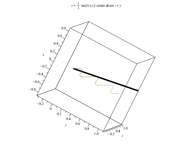
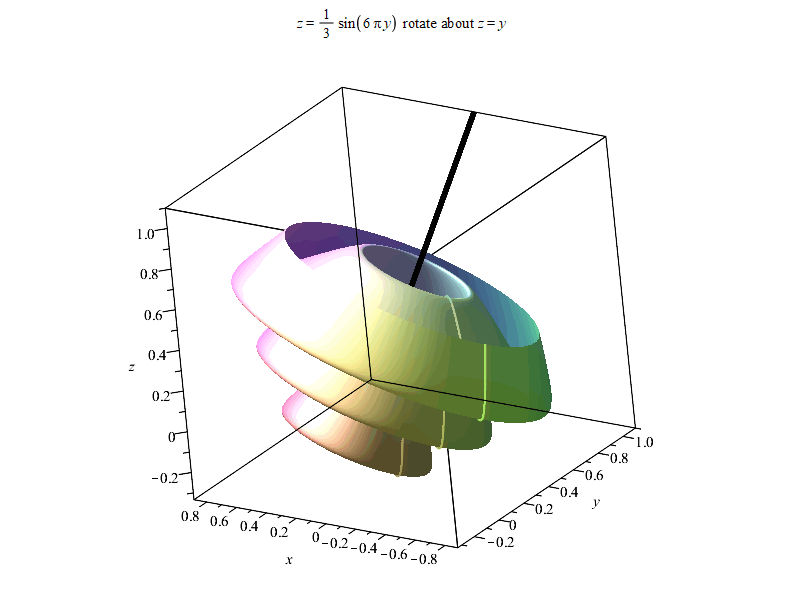
test_expr,test_k:=sin(Pi*6*y)/3,1:
#test_expr,test_k:=t->piecewise(t>=0 and t<=1/2,1/2-sqrt(1/4-t^2),t>1/2 and t<3/4,1/2,t>=3/4 and t<=1,2*t-1),1:
actual_expr:=[evalf(subs(k=test_k,rotate_point_down)),evalf(subs(k=test_k,rotate_point_up))]:
test_plot:=plot([test_expr,test_k*y],y=0..1,labels=['y','z'],title=typeset(z=test_expr," rotate about ",'z'=test_k*'y'));
#test_plot:=display(plot(test_expr,0..1),plot(test_k*y,y=0..1,labels=['y','z'],title=typeset(z=test_expr," rotate about ",'z'=test_k*'y')));
plotdata:=getdata(test_plot)[1,3]:

#create surfacedata
plot_y2d,plot_z2d:=convert(plotdata(..,1),list),convert(plotdata(..,2),list):
judge_subs_vector:=fastarray(plot_y2d*~test_k>=~plot_z2d,y2d=~plot_y2d,z2d=~plot_z2d):
surfacedata:=[seq(convert(fastarray(seq(evalf(map(location_adjust,judge_subs_vector,[actual_expr[1][ha],actual_expr[2][ha]])),ha=1..3)),list),tau in[seq(2*Pi/N*ha,ha=0..N)])]:

#create gif and import it
p1:=display(surfdata(surfacedata,labels=['x','y','z'],title=typeset(z=test_expr," rotate about ",'z'=test_k*'y'),style=surface),plot3d(y,x=0..0,y=0..1.1,thickness=5,color="red")):
display(display(seq(curve(surfacedata[ha],thickness=4),ha=1..N+1),insequence=true),p1,orientation=[-112,66,-167]);
Export(cat(filename,"curve_on_surface.gif"),%):
display(display(curve(surfacedata[1]),seq(surfdata(surfacedata[1..ha],style=surface),ha=2..N+1),insequence=true,labels=['x','y','z']),plot3d(y,x=0..0,y=0..1.1,thickness=5,color="red"),orientation=[152,5,166],title=typeset(z=test_expr," rotate about ",'z'=test_k*'y'));
Export(cat(filename,"surf.gif"),%):

#read some necessry packages and expressions and functions

用read笔法读取，filename前后保持一致，默认帧数是50。

#initial curve

写进三个测试函数，其中两个选择注释。第三个测试函数由于是分段函数，对应的是注释掉的test_plot。

#create surfacedata

这段代码可以好好学习，个人觉得帮助会比较大。因为她规避了for&if笔法，采用command~和map进行循环操作。

#create gif and import it

常规操作。重点体会surfdata绘制离散曲面图以及export如何输出图像。

以下是结果。由于输出时偷懒使用%表示上一个结果，Maple可能最后会报错

“Error, (in Export) exported file C:/Users/ysl-pc/Desktop/surf.gif could not be created”，但不影响输出结果~