昇思25天学习打卡营第5天|基础知识-网络构建

神经网络模型是由神经网络层和Tensor操作构成的，mindspore.nn提供了常见神经网络层的实现，在MindSpore中，Cell类是构建所有网络的基类，也是网络的基本单元。

一个神经网络模型表示为一个Cell，它由不同的子Cell构成。使用这样的嵌套结构，可以简单地使用面向对象编程的思维，对神经网络结构进行构建和管理。

下面我们将构建一个用于Mnist数据集分类的神经网络模型。

目录

环境

定义模型类

模型参数

---

环境

%%capture captured_output
# 实验环境已经预装了mindspore==2.2.14，如需更换mindspore版本，可更改下面mindspore的版本号
!pip uninstall mindspore -y
!pip install -i https://pypi.mirrors.ustc.edu.cn/simple mindspore==2.2.14

import mindspore
from mindspore import nn, ops

定义模型类

当我们定义神经网络时，可以继承nn.Cell类，在__init__方法中进行子Cell的实例化和状态管理，在construct方法中实现Tensor操作。

construct意为神经网络（计算图）构建

class Network(nn.Cell):
    def __init__(self):
        super().__init__()
        self.flatten = nn.Flatten()
        self.dense_relu_sequential = nn.SequentialCell(
            nn.Dense(28*28, 512, weight_init="normal", bias_init="zeros"),
            nn.ReLU(),
            nn.Dense(512, 512, weight_init="normal", bias_init="zeros"),
            nn.ReLU(),
            nn.Dense(512, 10, weight_init="normal", bias_init="zeros")
        )

    def construct(self, x):
        x = self.flatten(x)
        logits = self.dense_relu_sequential(x)
        return logits

其中：

1. nn.Flatten 

这个层的作用是将输入的多维数据（如图像）展平成一维数据，以便可以输入到全连接层（Dense层）中。这里假设输入数据是二维图像（例如，MNIST数据集中的28x28像素图像），展平后变为784维的向量。

实例化nn.Flatten层，将28x28的2D张量转换为784大小的连续数组。

# 构造一个shape为(3, 28, 28)的随机数据（3个28x28的图像）
input_image = ops.ones((3, 28, 28), mindspore.float32)
print(input_image.shape)

# 实例化nn.Flatten层，将28x28的2D张量转换为784大小的连续数组。
flatten = nn.Flatten()
flat_image = flatten(input_image)
print(flat_image.shape)

# (3, 784)

2. nn.Dense

nn.Dense为全连接层，其使用权重和偏差对输入进行线性变换。

# nn.Dense为全连接层，其使用权重和偏差对输入进行线性变换

layer1 = nn.Dense(in_channels=28*28, out_channels=20)
hidden1 = layer1(flat_image)
print(hidden1.shape)

# (3, 20)

3. nn.ReLU

nn.ReLU层给网络中加入非线性的激活函数，帮助神经网络学习各种复杂的特征。

print(f"Before ReLU: {hidden1}\n\n")
hidden1 = nn.ReLU()(hidden1)
print(f"After ReLU: {hidden1}")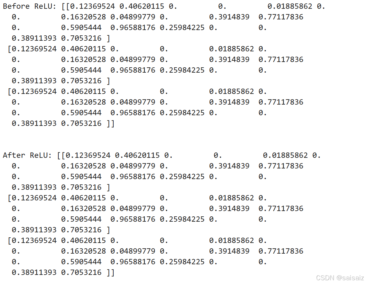

 

4. nn.SequentialCell

nn.SequentialCell是一个有序的Cell容器。输入Tensor将按照定义的顺序通过所有Cell。我们可以使用SequentialCell来快速组合构造一个神经网络模型

seq_modules = nn.SequentialCell(
    flatten,
    layer1,
    nn.ReLU(),
    nn.Dense(20, 10)
)

logits = seq_modules(input_image)
print(logits.shape)

# (3, 10)

 5. nn.Softmax

最后使用nn.Softmax将神经网络最后一个全连接层返回的logits的值缩放为[0, 1]，表示每个类别的预测概率。axis指定的维度数值和为1。

softmax = nn.Softmax(axis=1)
pred_probab = softmax(logits)

构建完成后，实例化Network对象，并查看其结构。

model = Network()
print(model)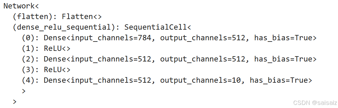

构造一个输入数据，直接调用模型，可以获得一个十维的Tensor输出，其包含每个类别的原始预测值。

model.construct()方法不可直接调用

X = ops.ones((1, 28, 28), mindspore.float32)
logits = model(X)
# print logits
logits

结果： 

其中：

input_image = ops.ones((3, 28, 28), mindspore.float32)
print(input_image.shape)

# (3, 28, 28)

构造一个shape为(3, 28, 28)的随机数据（3个28x28的图像），依次通过每一个神经网络层来观察其效果 

在此基础上，我们通过一个nn.Softmax层实例来获得预测概率。

pred_probab = nn.Softmax(axis=1)(logits)
y_pred = pred_probab.argmax(1)
print(f"Predicted class: {y_pred}")

# Predicted class: [4]

模型参数

网络内部神经网络层具有权重参数和偏置参数（如nn.Dense），这些参数会在训练过程中不断进行优化，可通过 model.parameters_and_names() 来获取参数名及对应的参数详情。

print(f"Model structure: {model}\n\n")

for name, param in model.parameters_and_names():
    print(f"Layer: {name}\nSize: {param.shape}\nValues : {param[:2]} \n")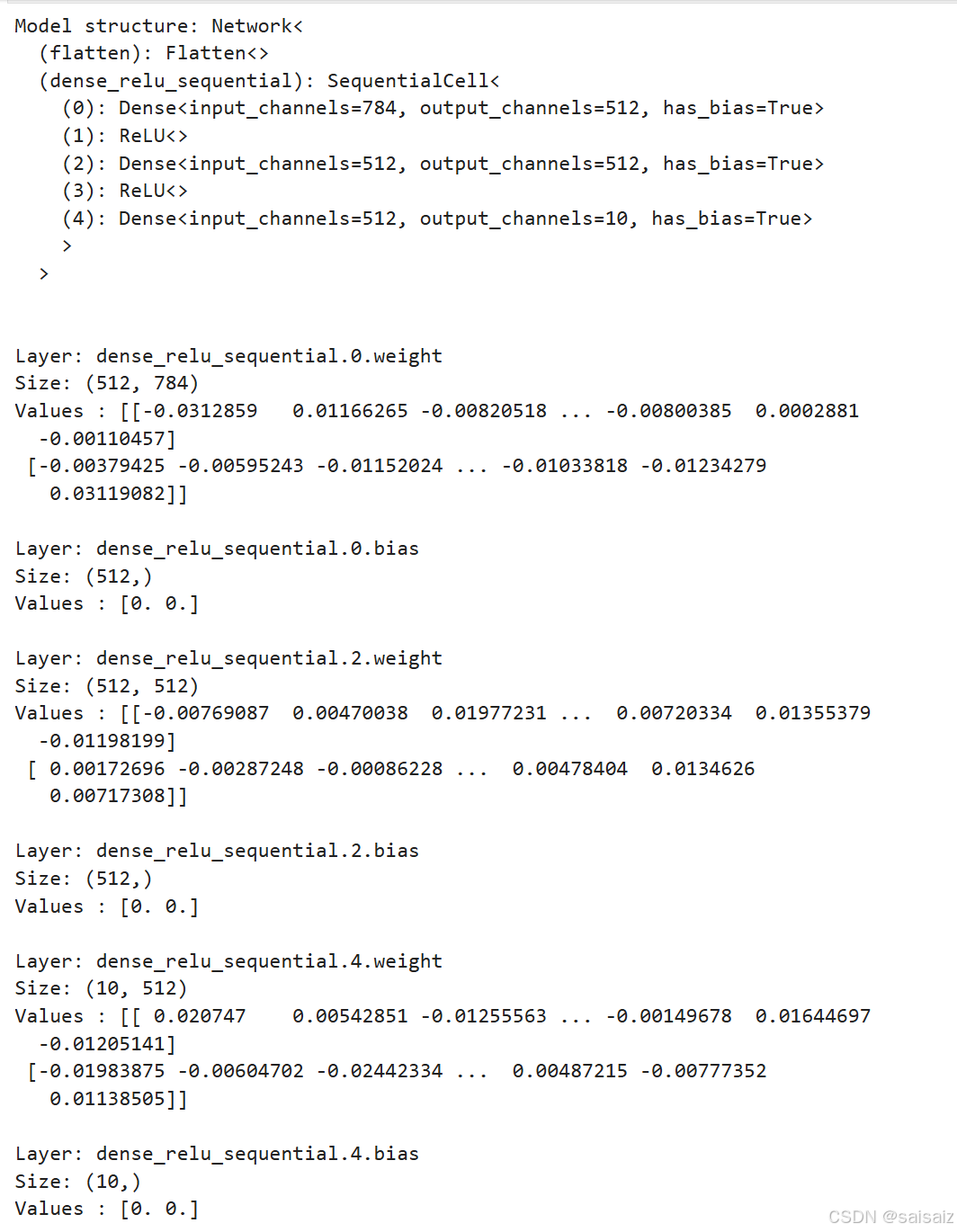

学习打卡时间