1_泰坦尼克号EDA

import pandas as pd 
import numpy as np
import os
import warnings
import seaborn as sns
import matplotlib.pyplot as plt
import missingno as msno

plt.rcParams['font.sans-serif']=['SimHei'] #用来正常显示中文标签
plt.rcParams['axes.unicode_minus'] = False #用来正常显示负号

warnings.filterwarnings('ignore')

#查看当前路径
os.getcwd()

'C:\\Develop\\python_project\\ML\\learning'

data = pd.read_csv(r'./data/train.csv', names=['乘客ID','是否幸存','仓位等级','姓名','性别','年龄','兄弟姐妹个数','父母子女个数','船票信息','票价','客舱','登船港口'],index_col='乘客ID',header=0)
data.head()

	是否幸存	仓位等级	姓名	性别	年龄	兄弟姐妹个数	父母子女个数	船票信息	票价	客舱	登船港口
乘客ID
1	0	3	Braund, Mr. Owen Harris	male	22.0	1	0	A/5 21171	7.2500	NaN	S
2	1	1	Cumings, Mrs. John Bradley (Florence Briggs Th...	female	38.0	1	0	PC 17599	71.2833	C85	C
3	1	3	Heikkinen, Miss. Laina	female	26.0	0	0	STON/O2. 3101282	7.9250	NaN	S
4	1	1	Futrelle, Mrs. Jacques Heath (Lily May Peel)	female	35.0	1	0	113803	53.1000	C123	S
5	0	3	Allen, Mr. William Henry	male	35.0	0	0	373450	8.0500	NaN	S

# data.to_csv(r'./data/train1.csv')

data.shape

(891, 11)

data.info(verbose=True)

<class 'pandas.core.frame.DataFrame'>
Int64Index: 891 entries, 1 to 891
Data columns (total 11 columns):
 #   Column  Non-Null Count  Dtype  
---  ------  --------------  -----  
 0   是否幸存    891 non-null    int64  
 1   仓位等级    891 non-null    int64  
 2   姓名      891 non-null    object 
 3   性别      891 non-null    object 
 4   年龄      714 non-null    float64
 5   兄弟姐妹个数  891 non-null    int64  
 6   父母子女个数  891 non-null    int64  
 7   船票信息    891 non-null    object 
 8   票价      891 non-null    float64
 9   客舱      204 non-null    object 
 10  登船港口    889 non-null    object 
dtypes: float64(2), int64(4), object(5)
memory usage: 83.5+ KB

data.describe()

	是否幸存	仓位等级	年龄	兄弟姐妹个数	父母子女个数	票价
count	891.000000	891.000000	714.000000	891.000000	891.000000	891.000000
mean	0.383838	2.308642	29.699118	0.523008	0.381594	32.204208
std	0.486592	0.836071	14.526497	1.102743	0.806057	49.693429
min	0.000000	1.000000	0.420000	0.000000	0.000000	0.000000
25%	0.000000	2.000000	20.125000	0.000000	0.000000	7.910400
50%	0.000000	3.000000	28.000000	0.000000	0.000000	14.454200
75%	1.000000	3.000000	38.000000	1.000000	0.000000	31.000000
max	1.000000	3.000000	80.000000	8.000000	6.000000	512.329200

data.describe(include='O')

	姓名	性别	船票信息	客舱	登船港口
count	891	891	891	204	889
unique	891	2	681	147	3
top	Mernagh, Mr. Robert	male	1601	G6	S
freq	1	577	7	4	644

#查看缺失值的情况
data.isnull().sum()

是否幸存        0
仓位等级        0
姓名          0
性别          0
年龄        177
兄弟姐妹个数      0
父母子女个数      0
船票信息        0
票价          0
客舱        687
登船港口        2
dtype: int64

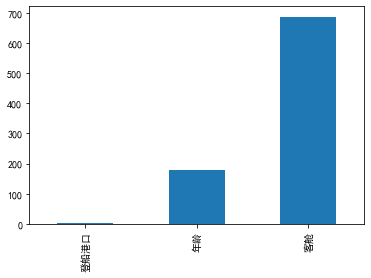
# nan可视化
missing = data.isnull().sum()
missing = missing[missing > 0]
missing.sort_values(inplace=True)
missing.plot.bar()

data['客舱'].value_counts()

G6             4
C23 C25 C27    4
B96 B98        4
F2             3
D              3
              ..
B78            1
A23            1
E63            1
C91            1
E36            1
Name: 客舱, Length: 147, dtype: int64

客舱是否和票价有相关。

PS：将客舱的首字母作为客舱等级的类别条件

from collections import Iterable
data['客舱等级']=data['客舱'].apply(lambda x : x[0] if isinstance(x,Iterable)  == True else np.nan)
data[['客舱','客舱等级']]

	客舱	客舱等级
乘客ID
1	NaN	NaN
2	C85	C
3	NaN	NaN
4	C123	C
5	NaN	NaN
...	...	...
887	NaN	NaN
888	B42	B
889	NaN	NaN
890	C148	C
891	NaN	NaN

891 rows × 2 columns

data['客舱等级'].value_counts()

C    59
B    47
D    33
E    32
A    15
F    13
G     4
T     1
Name: 客舱等级, dtype: int64

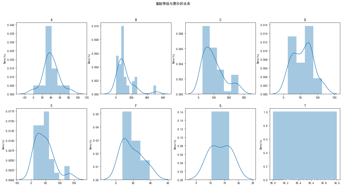
fig,axes=plt.subplots(2,4,figsize=(20, 10))  #创建一个1行三列的图片  
#设置主标题
fig.suptitle('客舱等级与票价的关系')
axes[0][0].set_title('A')
sns.distplot(data[['票价']].loc[data['客舱等级']=='A'],ax=axes[0,0]);
axes[0][1].set_title('B')
sns.distplot(data[['票价']].loc[data['客舱等级']=='B'],ax=axes[0,1]);
axes[0][2].set_title('C')
sns.distplot(data[['票价']].loc[data['客舱等级']=='C'],ax=axes[0,2]);
axes[0][3].set_title('D')
sns.distplot(data[['票价']].loc[data['客舱等级']=='D'],ax=axes[0,3]);
axes[1][0].set_title('E')
sns.distplot(data[['票价']].loc[data['客舱等级']=='E'],ax=axes[1,0]);
axes[1][1].set_title('F')
sns.distplot(data[['票价']].loc[data['客舱等级']=='F'],ax=axes[1,1]);
axes[1][2].set_title('G')
sns.distplot(data[['票价']].loc[data['客舱等级']=='G'],ax=axes[1,2]);
axes[1][3].set_title('T')
sns.distplot(data[['票价']].loc[data['客舱等级']=='T'],ax=axes[1,3]);

data[['性别','年龄','票价','客舱等级']].loc[data['客舱等级'].notna()]

	性别	年龄	票价	客舱等级
乘客ID
2	female	38.0	71.2833	C
4	female	35.0	53.1000	C
7	male	54.0	51.8625	E
11	female	4.0	16.7000	G
12	female	58.0	26.5500	C
...	...	...	...	...
872	female	47.0	52.5542	D
873	male	33.0	5.0000	B
880	female	56.0	83.1583	C
888	female	19.0	30.0000	B
890	male	26.0	30.0000	C

204 rows × 4 columns

for column in ["性别","登船港口"]:
    print("字段名",column)
    print("------------------")
    print(data[column].value_counts())

字段名 性别
------------------
male      577
female    314
Name: 性别, dtype: int64
字段名 登船港口
------------------
S    644
C    168
Q     77
Name: 登船港口, dtype: int64

data['性别_标识'] = data['性别'].map({'male': 1, 'female': 2})
data.head()

	是否幸存	仓位等级	姓名	性别	年龄	兄弟姐妹个数	父母子女个数	船票信息	票价	客舱	登船港口	客舱等级	性别_标识
乘客ID
1	0	3	Braund, Mr. Owen Harris	male	22.0	1	0	A/5 21171	7.2500	NaN	S	NaN	1
2	1	1	Cumings, Mrs. John Bradley (Florence Briggs Th...	female	38.0	1	0	PC 17599	71.2833	C85	C	C	2
3	1	3	Heikkinen, Miss. Laina	female	26.0	0	0	STON/O2. 3101282	7.9250	NaN	S	NaN	2
4	1	1	Futrelle, Mrs. Jacques Heath (Lily May Peel)	female	35.0	1	0	113803	53.1000	C123	S	C	2
5	0	3	Allen, Mr. William Henry	male	35.0	0	0	373450	8.0500	NaN	S	NaN	1

data['登船港口_标识']= data['登船港口'].map({'S': 1, 'C': 2, 'Q': 3})
data.head()

	是否幸存	仓位等级	姓名	性别	年龄	兄弟姐妹个数	父母子女个数	船票信息	票价	客舱	登船港口	客舱等级	性别_标识	登船港口_标识
乘客ID
1	0	3	Braund, Mr. Owen Harris	male	22.0	1	0	A/5 21171	7.2500	NaN	S	NaN	1	1.0
2	1	1	Cumings, Mrs. John Bradley (Florence Briggs Th...	female	38.0	1	0	PC 17599	71.2833	C85	C	C	2	2.0
3	1	3	Heikkinen, Miss. Laina	female	26.0	0	0	STON/O2. 3101282	7.9250	NaN	S	NaN	2	1.0
4	1	1	Futrelle, Mrs. Jacques Heath (Lily May Peel)	female	35.0	1	0	113803	53.1000	C123	S	C	2	1.0
5	0	3	Allen, Mr. William Henry	male	35.0	0	0	373450	8.0500	NaN	S	NaN	1	1.0

# data1 = data.loc[data['客舱等级'].notna()] #[['年龄','性别_标识','票价','仓位等级','客舱等级','登船港口_标识']]

data1=data.copy()

data1['年龄_分箱'] =pd.cut(data1['年龄'],[0,5,15,30,50,80],labels = False)

data1['票价_log'] = np.log(data1['票价'])

data1['票价_log'][np.isinf(data1['票价_log'])] = np.nan

data1.info()

<class 'pandas.core.frame.DataFrame'>
Int64Index: 891 entries, 1 to 891
Data columns (total 16 columns):
 #   Column   Non-Null Count  Dtype  
---  ------   --------------  -----  
 0   是否幸存     891 non-null    int64  
 1   仓位等级     891 non-null    int64  
 2   姓名       891 non-null    object 
 3   性别       891 non-null    object 
 4   年龄       714 non-null    float64
 5   兄弟姐妹个数   891 non-null    int64  
 6   父母子女个数   891 non-null    int64  
 7   船票信息     891 non-null    object 
 8   票价       891 non-null    float64
 9   客舱       204 non-null    object 
 10  登船港口     889 non-null    object 
 11  客舱等级     204 non-null    object 
 12  性别_标识    891 non-null    int64  
 13  登船港口_标识  889 non-null    float64
 14  年龄_分箱    714 non-null    float64
 15  票价_log   876 non-null    float64
dtypes: float64(5), int64(5), object(6)
memory usage: 118.3+ KB

#data1['年龄_分箱']=(data1['年龄_分箱'].notna()).astype(int)

# ## 特征与标签组合的散点可视化
# sns.pairplot(data=data1[['年龄','票价_log','客舱等级']],diag_kind='hist', hue= '客舱等级')
# plt.show()

客舱等级目前的分类效果比较差

# data1.groupby(['仓位等级','客舱等级','性别_标识'])['客舱等级'].count()

# data1.groupby(['仓位等级','客舱等级','性别_标识'])['票价'].mean()

票价是否和年龄性别仓位等级有关系。

data2=data1.loc[data['票价']==0]

data1=data1.loc[data1['票价']>0]
data1.info()

<class 'pandas.core.frame.DataFrame'>
Int64Index: 876 entries, 1 to 891
Data columns (total 16 columns):
 #   Column   Non-Null Count  Dtype  
---  ------   --------------  -----  
 0   是否幸存     876 non-null    int64  
 1   仓位等级     876 non-null    int64  
 2   姓名       876 non-null    object 
 3   性别       876 non-null    object 
 4   年龄       707 non-null    float64
 5   兄弟姐妹个数   876 non-null    int64  
 6   父母子女个数   876 non-null    int64  
 7   船票信息     876 non-null    object 
 8   票价       876 non-null    float64
 9   客舱       201 non-null    object 
 10  登船港口     874 non-null    object 
 11  客舱等级     201 non-null    object 
 12  性别_标识    876 non-null    int64  
 13  登船港口_标识  874 non-null    float64
 14  年龄_分箱    707 non-null    float64
 15  票价_log   876 non-null    float64
dtypes: float64(5), int64(5), object(6)
memory usage: 116.3+ KB

data1[['年龄','性别_标识','仓位等级','年龄_分箱','登船港口_标识','票价','票价_log']]

	年龄	性别_标识	仓位等级	年龄_分箱	登船港口_标识	票价	票价_log
乘客ID
1	22.0	1	3	2.0	1.0	7.2500	1.981001
2	38.0	2	1	3.0	2.0	71.2833	4.266662
3	26.0	2	3	2.0	1.0	7.9250	2.070022
4	35.0	2	1	3.0	1.0	53.1000	3.972177
5	35.0	1	3	3.0	1.0	8.0500	2.085672
...	...	...	...	...	...	...	...
887	27.0	1	2	2.0	1.0	13.0000	2.564949
888	19.0	2	1	2.0	1.0	30.0000	3.401197
889	NaN	2	3	NaN	1.0	23.4500	3.154870
890	26.0	1	1	2.0	2.0	30.0000	3.401197
891	32.0	1	3	3.0	3.0	7.7500	2.047693

876 rows × 7 columns

data1['票价'].value_counts()

8.0500     43
13.0000    42
7.8958     38
7.7500     34
26.0000    31
           ..
32.3208     1
13.8583     1
7.6292      1
15.0500     1
8.6833      1
Name: 票价, Length: 247, dtype: int64

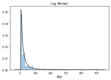
## 1) 总体分布概况（无界约翰逊分布等）
import scipy.stats as st
y = data1['票价']
plt.figure(1); plt.title('Johnson SU')
sns.distplot(y, kde=False, fit=st.johnsonsu)
plt.figure(2); plt.title('Normal')
sns.distplot(y, kde=False, fit=st.norm)
plt.figure(3); plt.title('Log Normal')
sns.distplot(y, kde=False, fit=st.lognorm)

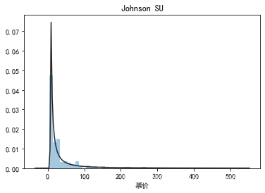
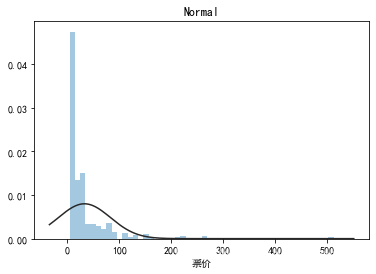
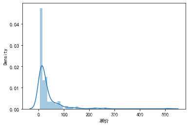
## 2) 查看skewness and kurtosis
sns.distplot(data1['票价']);
print("Skewness: %f" % data1['票价'].skew())
print("Kurtosis: %f" % data1['票价'].kurt())

Skewness: 4.770117
Kurtosis: 33.094179

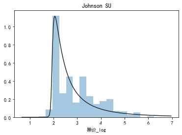
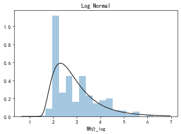
y = data1['票价_log']
plt.figure(1); plt.title('Johnson SU')
sns.distplot(y, kde=False, fit=st.johnsonsu)
plt.figure(2); plt.title('Normal')
sns.distplot(y, kde=False, fit=st.norm)
plt.figure(3); plt.title('Log Normal')
sns.distplot(y, kde=False, fit=st.lognorm)

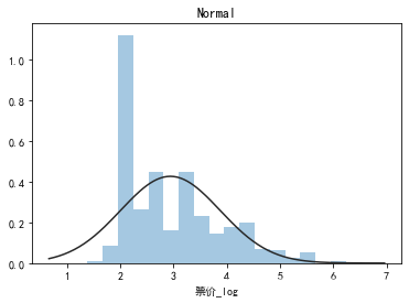
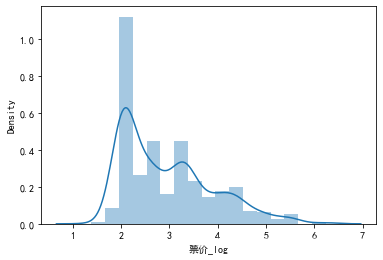
## 2) 查看skewness and kurtosis
sns.distplot(data1['票价_log']);
print("Skewness: %f" % data1['票价_log'].skew())
print("Kurtosis: %f" % data1['票价_log'].kurt())

Skewness: 0.901272
Kurtosis: 0.092646

data1.skew(), data1.kurt()

(是否幸存       0.454980
 仓位等级      -0.645700
 年龄         0.397549
 兄弟姐妹个数     3.663054
 父母子女个数     2.719314
 票价         4.770117
 性别_标识      0.591376
 登船港口_标识    1.513679
 年龄_分箱     -0.509732
 票价_log     0.901272
 dtype: float64,
 是否幸存       -1.797101
 仓位等级       -1.264175
 年龄          0.181680
 兄弟姐妹个数     17.569865
 父母子女个数      9.571814
 票价         33.094179
 性别_标识      -1.654057
 登船港口_标识     1.009103
 年龄_分箱       0.556544
 票价_log      0.092646
 dtype: float64)

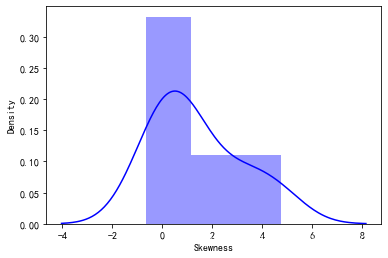
sns.distplot(data1.skew(),color='blue',axlabel ='Skewness')

sns.distplot(data1.kurt(),color='orange',axlabel ='Kurtness')

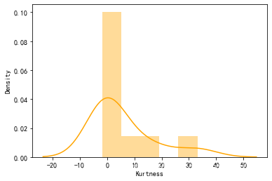
使用log对目标票价处理后,偏值和峰值下降到0.96,0.24总体属于正态分布,数据正偏右尾

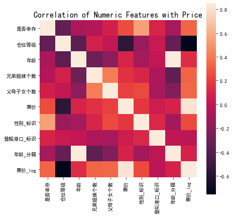
## 1) 相关性分析
price_numeric = data1
correlation = price_numeric.corr()
print(correlation['票价_log'].sort_values(ascending = False),'\n')

票价_log     1.000000
票价         0.817386
父母子女个数     0.339180
是否幸存       0.325452
兄弟姐妹个数     0.324373
性别_标识      0.247711
年龄         0.135352
年龄_分箱      0.091907
登船港口_标识   -0.012083
仓位等级      -0.754893
Name: 票价_log, dtype: float64 

f , ax = plt.subplots(figsize = (7, 7))

plt.title('Correlation of Numeric Features with Price',y=1,size=16)

sns.heatmap(correlation,square = True,  vmax=0.85)

# 对类别特征进行 OneEncoder  '年龄_分箱','性别_标识','仓位等级','登船港口_标识','票价_log'
data1 = pd.get_dummies(data1, columns=['年龄_分箱', '性别_标识', '仓位等级', '登船港口_标识'])

# 对类别特征进行 OneEncoder  '年龄_分箱','性别_标识','仓位等级','登船港口_标识','票价_log'
data2 = pd.get_dummies(data2, columns=['年龄_分箱', '性别_标识', '仓位等级', '登船港口_标识'])

data1.info()

<class 'pandas.core.frame.DataFrame'>
Int64Index: 876 entries, 1 to 891
Data columns (total 25 columns):
 #   Column       Non-Null Count  Dtype  
---  ------       --------------  -----  
 0   是否幸存         876 non-null    int64  
 1   姓名           876 non-null    object 
 2   性别           876 non-null    object 
 3   年龄           707 non-null    float64
 4   兄弟姐妹个数       876 non-null    int64  
 5   父母子女个数       876 non-null    int64  
 6   船票信息         876 non-null    object 
 7   票价           876 non-null    float64
 8   客舱           201 non-null    object 
 9   登船港口         874 non-null    object 
 10  客舱等级         201 non-null    object 
 11  票价_log       876 non-null    float64
 12  年龄_分箱_0.0    876 non-null    uint8  
 13  年龄_分箱_1.0    876 non-null    uint8  
 14  年龄_分箱_2.0    876 non-null    uint8  
 15  年龄_分箱_3.0    876 non-null    uint8  
 16  年龄_分箱_4.0    876 non-null    uint8  
 17  性别_标识_1      876 non-null    uint8  
 18  性别_标识_2      876 non-null    uint8  
 19  仓位等级_1       876 non-null    uint8  
 20  仓位等级_2       876 non-null    uint8  
 21  仓位等级_3       876 non-null    uint8  
 22  登船港口_标识_1.0  876 non-null    uint8  
 23  登船港口_标识_2.0  876 non-null    uint8  
 24  登船港口_标识_3.0  876 non-null    uint8  
dtypes: float64(3), int64(3), object(6), uint8(13)
memory usage: 100.1+ KB

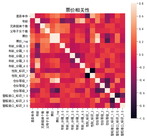
correlation = data1.corr()
f , ax = plt.subplots(figsize = (7, 7))
plt.title('票价相关性',y=1,size=16)
sns.heatmap(correlation,square = True,  vmax=0.8)

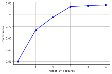
# k_feature 太大会很难跑，没服务器，所以提前 interrupt 了
from mlxtend.feature_selection import SequentialFeatureSelector as SFS
from sklearn.linear_model import LinearRegression
sfs = SFS(LinearRegression(),
           k_features=6,
           forward=True,
           floating=False,
           scoring = 'r2',
           cv = 0)
x = data1.drop(['票价','票价_log'], axis=1)
numerical_cols = x.select_dtypes(exclude = 'object').columns
x = x[numerical_cols]
x = x.fillna(0)
y = data1['票价_log'].fillna(0)
sfs.fit(x, y)
sfs.k_feature_names_ 

('兄弟姐妹个数', '父母子女个数', '性别_标识_1', '仓位等级_1', '仓位等级_2', '登船港口_标识_2.0')

from mlxtend.plotting import plot_sequential_feature_selection as plot_sfs
import matplotlib.pyplot as plt
fig1 = plot_sfs(sfs.get_metric_dict(), kind='std_dev')
plt.grid()
plt.show()

#将特征分类
#数字特征：'乘客ID','年龄','兄弟姐妹个数','父母子女个数','票价'
#类别特征：'仓位等级','性别','客舱','登船港口'
#文本型特征：'姓名','船票信息'
#目标：'是否幸存'

data1.to_csv('./data/train1.csv',encoding='utf_8_sig')

from sklearn.model_selection import train_test_split
x_train,x_test,y_train,y_test=train_test_split(data1[['兄弟姐妹个数', '父母子女个数', '性别_标识_1', '仓位等级_1', '仓位等级_3', '登船港口_标识_2.0']],
                                               data1['票价_log'],train_size=0.8)  #自动建立训练及测试 数据集函数，其中train_size=0.8为分割比例

print('x原始数据',data1[['兄弟姐妹个数', '父母子女个数', '性别_标识_1', '仓位等级_1', '仓位等级_3', '登船港口_标识_2.0']].shape,
     'x训练数据',x_train.shape,
     'x测试数据',x_test.shape,)
print('y原始数据',data1['票价_log'].shape,
     'y训练数据',y_train.shape,
     'y测试数据',y_test.shape,)

x原始数据 (876, 6) x训练数据 (700, 6) x测试数据 (176, 6)
y原始数据 (876,) y训练数据 (700,) y测试数据 (176,)

from sklearn.linear_model import LinearRegression
model= LinearRegression()
model.fit(x_train[['兄弟姐妹个数', '父母子女个数', '性别_标识_1', '仓位等级_1', '仓位等级_3', '登船港口_标识_2.0']],y_train)   #sklearn里的model.fit(X,y) 中的X，y必须是矩阵形式 

LinearRegression()

x_train=x_train.values

y_train=y_train.values

#第1步：导入线性回归
from sklearn.linear_model import LinearRegression
# 第2步：创建模型：线性回归
model = LinearRegression()
#第3步：训练模型
model.fit(x_train , y_train)

LinearRegression()

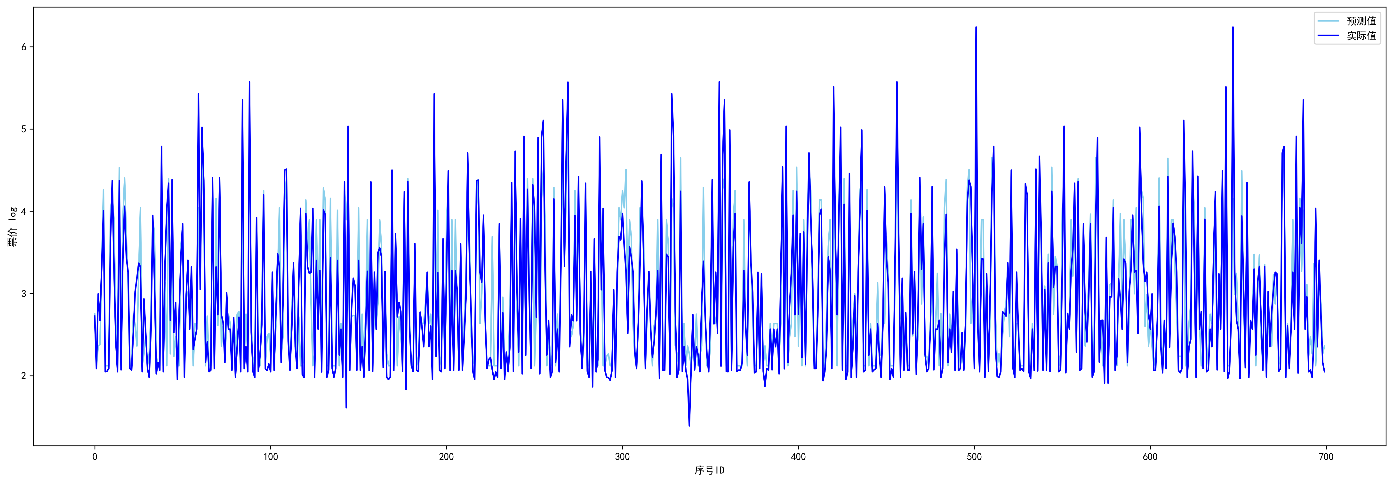
#训练数据的预测值
y_train_pred = model.predict(x_train)

plt.figure(dpi=300,figsize=(24,8))
plt.plot([i for  i in range(700)], y_train_pred,  color='skyblue', label='预测值')
plt.plot([i for  i in range(700)], y_train, color='blue', label='实际值')
plt.legend()
 
plt.xlabel('序号ID')
plt.ylabel('票价_log')
plt.show()

五折交叉验证&&均方误差&&平均绝对误差

from sklearn.model_selection import cross_val_score
from sklearn.metrics import mean_absolute_error,  make_scorer

def log_transfer(func):
    def wrapper(y, yhat):
        result = func(np.log(y), np.nan_to_num(np.log(yhat)))
        return result
    return wrapper

scores = cross_val_score(model, X=x_train, y=y_train, verbose=1, cv = 5, scoring=make_scorer(log_transfer(mean_absolute_error)))

[Parallel(n_jobs=1)]: Using backend SequentialBackend with 1 concurrent workers.
[Parallel(n_jobs=1)]: Done   5 out of   5 | elapsed:    0.0s finished

print('AVG:', np.mean(scores))

AVG: 0.09158952675993322

scores = cross_val_score(model, X=x_train, y=y_train_pred, verbose=1, cv = 5, scoring=make_scorer(mean_absolute_error))

[Parallel(n_jobs=1)]: Using backend SequentialBackend with 1 concurrent workers.
[Parallel(n_jobs=1)]: Done   5 out of   5 | elapsed:    0.0s finished

print('AVG:', np.mean(scores))

AVG: 1.4134725136370564e-15

scores = pd.DataFrame(scores.reshape(1,-1))
scores.columns = ['cv' + str(x) for x in range(1, 6)]
scores.index = ['平均绝对误差MAE']
scores

	cv1	cv2	cv3	cv4	cv5
平均绝对误差MAE	1.049954e-15	2.531308e-15	6.756500e-16	1.091191e-15	1.719260e-15

from sklearn.metrics import mean_squared_error
MSE = mean_squared_error(y_train, y_train_pred)
print('均方误差',MSE)

均方误差 0.17890857693897988

data2.info()#

<class 'pandas.core.frame.DataFrame'>
Int64Index: 15 entries, 180 to 823
Data columns (total 19 columns):
 #   Column       Non-Null Count  Dtype  
---  ------       --------------  -----  
 0   是否幸存         15 non-null     int64  
 1   姓名           15 non-null     object 
 2   性别           15 non-null     object 
 3   年龄           7 non-null      float64
 4   兄弟姐妹个数       15 non-null     int64  
 5   父母子女个数       15 non-null     int64  
 6   船票信息         15 non-null     object 
 7   票价           15 non-null     float64
 8   客舱           3 non-null      object 
 9   登船港口         15 non-null     object 
 10  客舱等级         3 non-null      object 
 11  票价_log       0 non-null      float64
 12  年龄_分箱_2.0    15 non-null     uint8  
 13  年龄_分箱_3.0    15 non-null     uint8  
 14  性别_标识_1      15 non-null     uint8  
 15  仓位等级_1       15 non-null     uint8  
 16  仓位等级_2       15 non-null     uint8  
 17  仓位等级_3       15 non-null     uint8  
 18  登船港口_标识_1.0  15 non-null     uint8  
dtypes: float64(3), int64(3), object(6), uint8(7)
memory usage: 1.6+ KB

data2['登船港口_标识_2.0']=0

data2_pred = model.predict(data2[['兄弟姐妹个数', '父母子女个数', '性别_标识_1', '仓位等级_1', '仓位等级_3', '登船港口_标识_2.0']])

data2_pred,np.exp(data2_pred)

(array([2.12092784, 3.8968038 , 2.12092784, 2.63339506, 2.12092784,
        2.63339506, 2.63339506, 2.63339506, 2.12092784, 3.8968038 ,
        2.63339506, 2.63339506, 3.8968038 , 3.8968038 , 3.8968038 ]),
 array([ 8.33887105, 49.24480131,  8.33887105, 13.92095222,  8.33887105,
        13.92095222, 13.92095222, 13.92095222,  8.33887105, 49.24480131,
        13.92095222, 13.92095222, 49.24480131, 49.24480131, 49.24480131]))

pd.DataFrame(data2_pred,columns=['票价'])

	票价
0	2.120928
1	3.896804
2	2.120928
3	2.633395
4	2.120928
5	2.633395
6	2.633395
7	2.633395
8	2.120928
9	3.896804
10	2.633395
11	2.633395
12	3.896804
13	3.896804
14	3.896804

pd.DataFrame(np.exp(data2_pred),columns=['票价'])

	票价
0	8.338871
1	49.244801
2	8.338871
3	13.920952
4	8.338871
5	13.920952
6	13.920952
7	13.920952
8	8.338871
9	49.244801
10	13.920952
11	13.920952
12	49.244801
13	49.244801
14	49.244801

del data2['票价']

data2.reset_index()

	乘客ID	是否幸存	姓名	性别	年龄	兄弟姐妹个数	父母子女个数	船票信息	客舱	登船港口	客舱等级	票价_log	年龄_分箱_2.0	年龄_分箱_3.0	性别_标识_1	仓位等级_1	仓位等级_2	仓位等级_3	登船港口_标识_1.0	登船港口_标识_2.0
0	180	0	Leonard, Mr. Lionel	male	36.0	0	0	LINE	NaN	S	NaN	NaN	0	1	1	0	0	1	1	0
1	264	0	Harrison, Mr. William	male	40.0	0	0	112059	B94	S	B	NaN	0	1	1	1	0	0	1	0
2	272	1	Tornquist, Mr. William Henry	male	25.0	0	0	LINE	NaN	S	NaN	NaN	1	0	1	0	0	1	1	0
3	278	0	Parkes, Mr. Francis "Frank"	male	NaN	0	0	239853	NaN	S	NaN	NaN	0	0	1	0	1	0	1	0
4	303	0	Johnson, Mr. William Cahoone Jr	male	19.0	0	0	LINE	NaN	S	NaN	NaN	1	0	1	0	0	1	1	0
5	414	0	Cunningham, Mr. Alfred Fleming	male	NaN	0	0	239853	NaN	S	NaN	NaN	0	0	1	0	1	0	1	0
6	467	0	Campbell, Mr. William	male	NaN	0	0	239853	NaN	S	NaN	NaN	0	0	1	0	1	0	1	0
7	482	0	Frost, Mr. Anthony Wood "Archie"	male	NaN	0	0	239854	NaN	S	NaN	NaN	0	0	1	0	1	0	1	0
8	598	0	Johnson, Mr. Alfred	male	49.0	0	0	LINE	NaN	S	NaN	NaN	0	1	1	0	0	1	1	0
9	634	0	Parr, Mr. William Henry Marsh	male	NaN	0	0	112052	NaN	S	NaN	NaN	0	0	1	1	0	0	1	0
10	675	0	Watson, Mr. Ennis Hastings	male	NaN	0	0	239856	NaN	S	NaN	NaN	0	0	1	0	1	0	1	0
11	733	0	Knight, Mr. Robert J	male	NaN	0	0	239855	NaN	S	NaN	NaN	0	0	1	0	1	0	1	0
12	807	0	Andrews, Mr. Thomas Jr	male	39.0	0	0	112050	A36	S	A	NaN	0	1	1	1	0	0	1	0
13	816	0	Fry, Mr. Richard	male	NaN	0	0	112058	B102	S	B	NaN	0	0	1	1	0	0	1	0
14	823	0	Reuchlin, Jonkheer. John George	male	38.0	0	0	19972	NaN	S	NaN	NaN	0	1	1	1	0	0	1	0

data2=pd.concat([data2.reset_index(),pd.DataFrame(np.exp(data2_pred),columns=['票价'])],axis=1)

data2['票价_log'] = np.log(data2['票价'])

data2.set_index(["乘客ID"], inplace=True)

data2

	是否幸存	姓名	性别	年龄	兄弟姐妹个数	父母子女个数	船票信息	客舱	登船港口	客舱等级	票价_log	年龄_分箱_2.0	年龄_分箱_3.0	性别_标识_1	仓位等级_1	仓位等级_2	仓位等级_3	登船港口_标识_1.0	登船港口_标识_2.0	票价
乘客ID
180	0	Leonard, Mr. Lionel	male	36.0	0	0	LINE	NaN	S	NaN	2.120928	0	1	1	0	0	1	1	0	8.338871
264	0	Harrison, Mr. William	male	40.0	0	0	112059	B94	S	B	3.896804	0	1	1	1	0	0	1	0	49.244801
272	1	Tornquist, Mr. William Henry	male	25.0	0	0	LINE	NaN	S	NaN	2.120928	1	0	1	0	0	1	1	0	8.338871
278	0	Parkes, Mr. Francis "Frank"	male	NaN	0	0	239853	NaN	S	NaN	2.633395	0	0	1	0	1	0	1	0	13.920952
303	0	Johnson, Mr. William Cahoone Jr	male	19.0	0	0	LINE	NaN	S	NaN	2.120928	1	0	1	0	0	1	1	0	8.338871
414	0	Cunningham, Mr. Alfred Fleming	male	NaN	0	0	239853	NaN	S	NaN	2.633395	0	0	1	0	1	0	1	0	13.920952
467	0	Campbell, Mr. William	male	NaN	0	0	239853	NaN	S	NaN	2.633395	0	0	1	0	1	0	1	0	13.920952
482	0	Frost, Mr. Anthony Wood "Archie"	male	NaN	0	0	239854	NaN	S	NaN	2.633395	0	0	1	0	1	0	1	0	13.920952
598	0	Johnson, Mr. Alfred	male	49.0	0	0	LINE	NaN	S	NaN	2.120928	0	1	1	0	0	1	1	0	8.338871
634	0	Parr, Mr. William Henry Marsh	male	NaN	0	0	112052	NaN	S	NaN	3.896804	0	0	1	1	0	0	1	0	49.244801
675	0	Watson, Mr. Ennis Hastings	male	NaN	0	0	239856	NaN	S	NaN	2.633395	0	0	1	0	1	0	1	0	13.920952
733	0	Knight, Mr. Robert J	male	NaN	0	0	239855	NaN	S	NaN	2.633395	0	0	1	0	1	0	1	0	13.920952
807	0	Andrews, Mr. Thomas Jr	male	39.0	0	0	112050	A36	S	A	3.896804	0	1	1	1	0	0	1	0	49.244801
816	0	Fry, Mr. Richard	male	NaN	0	0	112058	B102	S	B	3.896804	0	0	1	1	0	0	1	0	49.244801
823	0	Reuchlin, Jonkheer. John George	male	38.0	0	0	19972	NaN	S	NaN	3.896804	0	1	1	1	0	0	1	0	49.244801

缺失的票价补充完成

data1.info()

<class 'pandas.core.frame.DataFrame'>
Int64Index: 876 entries, 1 to 891
Data columns (total 25 columns):
 #   Column       Non-Null Count  Dtype  
---  ------       --------------  -----  
 0   是否幸存         876 non-null    int64  
 1   姓名           876 non-null    object 
 2   性别           876 non-null    object 
 3   年龄           707 non-null    float64
 4   兄弟姐妹个数       876 non-null    int64  
 5   父母子女个数       876 non-null    int64  
 6   船票信息         876 non-null    object 
 7   票价           876 non-null    float64
 8   客舱           201 non-null    object 
 9   登船港口         874 non-null    object 
 10  客舱等级         201 non-null    object 
 11  票价_log       876 non-null    float64
 12  年龄_分箱_0.0    876 non-null    uint8  
 13  年龄_分箱_1.0    876 non-null    uint8  
 14  年龄_分箱_2.0    876 non-null    uint8  
 15  年龄_分箱_3.0    876 non-null    uint8  
 16  年龄_分箱_4.0    876 non-null    uint8  
 17  性别_标识_1      876 non-null    uint8  
 18  性别_标识_2      876 non-null    uint8  
 19  仓位等级_1       876 non-null    uint8  
 20  仓位等级_2       876 non-null    uint8  
 21  仓位等级_3       876 non-null    uint8  
 22  登船港口_标识_1.0  876 non-null    uint8  
 23  登船港口_标识_2.0  876 non-null    uint8  
 24  登船港口_标识_3.0  876 non-null    uint8  
dtypes: float64(3), int64(3), object(6), uint8(13)
memory usage: 140.1+ KB

data2.info()

<class 'pandas.core.frame.DataFrame'>
Int64Index: 15 entries, 180 to 823
Data columns (total 20 columns):
 #   Column       Non-Null Count  Dtype  
---  ------       --------------  -----  
 0   是否幸存         15 non-null     int64  
 1   姓名           15 non-null     object 
 2   性别           15 non-null     object 
 3   年龄           7 non-null      float64
 4   兄弟姐妹个数       15 non-null     int64  
 5   父母子女个数       15 non-null     int64  
 6   船票信息         15 non-null     object 
 7   客舱           3 non-null      object 
 8   登船港口         15 non-null     object 
 9   客舱等级         3 non-null      object 
 10  票价_log       15 non-null     float64
 11  年龄_分箱_2.0    15 non-null     uint8  
 12  年龄_分箱_3.0    15 non-null     uint8  
 13  性别_标识_1      15 non-null     uint8  
 14  仓位等级_1       15 non-null     uint8  
 15  仓位等级_2       15 non-null     uint8  
 16  仓位等级_3       15 non-null     uint8  
 17  登船港口_标识_1.0  15 non-null     uint8  
 18  登船港口_标识_2.0  15 non-null     int64  
 19  票价           15 non-null     float64
dtypes: float64(3), int64(4), object(6), uint8(7)
memory usage: 1.7+ KB