


设计实验内容
在设定的语料集上进行说话人确认实验
验证超参对性能的影响(易)
验证新的改动对性能的影响(难)
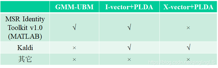
方法一览:
我有别的事情要忙,所以做了个最简单的,傻瓜式实验……
GMM-UBM方法,
数据 (不知道什么时候失效,链接不要扩散出去。。。)
PS:失效了不要联系我补上,我懒得传,给钱我也懒……
project数据及代码链接:https://pan.baidu.com/s/1V26dSAUZ6ca2FrPzmsK2Kg
提取码:c1q2
117名说话人,男性
每名说话人几百条语料
Wav格式,16kHz 16bit
语料很多很短,不足3秒
关于代码:其实给出的demo已经写的很清楚了,下面这个代码推荐使用!
%{
This is a demo on how to use the Identity Toolbox for GMM-UBM based speaker
recognition. A small scale task has been designed using artificially
generated features for 20 speakers. Each speaker has 10 sessions
(channels) and each session is 1000 frames long (10 seconds assuming 10 ms
frame increments).
There are 4 steps involved:
1. training a UBM from background data
2. MAP adapting speaker models from the UBM using enrollment data
3. scoring verification trials
4. computing the performance measures (e.g., confusion matrix and EER)
Note: given the relatively small size of the task, we can load all the data
and models into memory. This, however, may not be practical for large scale
tasks (or on machines with a limited memory). In such cases, the parameters
should be saved to the disk.
Malcolm Slaney <mslaney@microsoft.com>
Omid Sadjadi <s.omid.sadjadi@gmail.com>
Microsoft Research, Conversational Systems Research Center
%}
%
%%
% Step0: Set the parameters of the experiment
nSpeakers = 20;
nDims = 13; % dimensionality of feature vectors
nMixtures = 32; % How many mixtures used to generate data
nChannels = 10; % Number of channels (sessions) per speaker
nFrames = 1000; % Frames per speaker (10 seconds assuming 100 Hz)
nWorkers = 1; % Number of parfor workers, if available
% Pick random centers for all the mixtures.
mixtureVariance = .10;
channelVariance = .05;
mixtureCenters = randn(nDims, nMixtures, nSpeakers);
channelCenters = randn(nDims, nMixtures, nSpeakers, nChannels)*.1;
trainSpeakerData = cell(nSpeakers, nChannels);
testSpeakerData = cell(nSpeakers, nChannels);
speakerID = zeros(nSpeakers, nChannels);
% Create the random data. Both training and testing data have the same
% layout.
for s=1:nSpeakers
trainSpeechData = zeros(nDims, nMixtures);
testSpeechData = zeros(nDims, nMixtures);
for c=1:nChannels
for m=1:nMixtures
% Create data from mixture m for speaker s
frameIndices = m:nMixtures:nFrames;
nMixFrames = length(frameIndices);
trainSpeechData(:,frameIndices) = ...
randn(nDims, nMixFrames)*sqrt(mixtureVariance) + ...
repmat(mixtureCenters(:,m,s),1,nMixFrames) + ...
repmat(channelCenters(:,m,s,c),1,nMixFrames);
testSpeechData(:,frameIndices) = ...
randn(nDims, nMixFrames)*sqrt(mixtureVariance) + ...
repmat(mixtureCenters(:,m,s),1,nMixFrames) + ...
repmat(channelCenters(:,m,s,c),1,nMixFrames);
end
trainSpeakerData{s, c} = trainSpeechData;
testSpeakerData{s, c} = testSpeechData;
speakerID(s,c) = s; % Keep track of who this is
end
end
%%
% Step1: Create the universal background model from all the training speaker data
nmix = nMixtures; % In this case, we know the # of mixtures needed
final_niter = 10;
ds_factor = 1;
ubm = gmm_em(trainSpeakerData(:), nmix, final_niter, ds_factor, nWorkers);
%%
% Step2: Now adapt the UBM to each speaker to create GMM speaker model.
map_tau = 10.0;
config = 'mwv';
gmm = cell(nSpeakers, 1);
for s=1:nSpeakers
gmm{s} = mapAdapt(trainSpeakerData(s, :), ubm, map_tau, config);
end
%%
% Step3: Now calculate the score for each model versus each speaker's data.
% Generate a list that tests each model (first column) against all the
% testSpeakerData.
trials = zeros(nSpeakers*nChannels*nSpeakers, 2);
answers = zeros(nSpeakers*nChannels*nSpeakers, 1);
for ix = 1 : nSpeakers,
b = (ix-1)*nSpeakers*nChannels + 1;
e = b + nSpeakers*nChannels - 1;
trials(b:e, :) = [ix * ones(nSpeakers*nChannels, 1), (1:nSpeakers*nChannels)'];
answers((ix-1)*nChannels+b : (ix-1)*nChannels+b+nChannels-1) = 1;
end
gmmScores = score_gmm_trials(gmm, reshape(testSpeakerData', nSpeakers*nChannels,1), trials, ubm);
%%
% Step4: Now compute the EER and plot the DET curve and confusion matrix
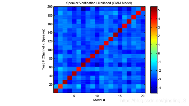
imagesc(reshape(gmmScores,nSpeakers*nChannels, nSpeakers))
title('Speaker Verification Likelihood (GMM Model)');
ylabel('Test # (Channel x Speaker)'); xlabel('Model #');
colorbar; drawnow; axis xy
figure
eer = compute_eer(gmmScores, answers, true);
下面是操作步骤:
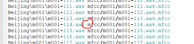
1.得到了一大堆wav文件
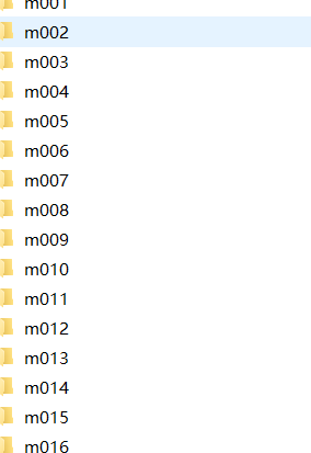
打开是这样的:
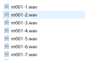
头疼,这一堆wav还得先转化为mfcc特征才行啊,
下载一个htk(官网需要先注册),我用的版本是htk3.4
安装和使用流程在这里,我就不赘述了,有出现问题的可以在下面留言。
https://blog.youkuaiyun.com/qq_38161654/article/details/81172741
注意:htk的编译已经加入到了visual studio中,所以你如果有了visual studio可以用他的包直接编译,地址是:
2017的VisualStudio上面bin的地址 在:C:\Program Files (x86)\Microsoft Visual Studio\2017\Community\VC\Auxiliary\Build
有出现问题的可以在下面留言。
上面的wav转化为mfcc需要两个文件:

hcopy.scp 里面长这样:
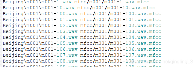
这里我是用的是htk的相对地址,你也可以生成绝对地址。
由于文件很多,又在不同文件夹里,我使用了下面的代码来生成这个hcopy.scp文件
#!/usr/bin/python
# -*- coding:utf8 -*-

import os

# 遍历指定目录,显示目录下的所有文件名
def eachFile(filepath,f):
    pathDir = os.listdir(filepath)
    for allDir in pathDir:
        child = os.path.join('%s%s' % (filepath, allDir))
        names=allDir.split("-")
        if os.path.isfile(child) and allDir[0]=='m':
              f.write((child+" "+child+".mfcc").replace('D:\\说话人确认项目资源文件\\my-htk\\', ''))
        if(allDir[0]=='m' and os.path.isdir(child)):
            eachFile(child+"\\",f)

if __name__ == '__main__':
    f = open('D:\\说话人确认项目资源文件\\my-htk\\hcopy.scp', 'w')
    filePath = "D:\\说话人确认项目资源文件\\my-htk\\Beijing\\"
    eachFile(filePath,f)
生成的文件放在D:\\说话人确认项目资源文件\\my-htk\\hcopy.scp里面,路径问题你们自己解决,这不是重点。生成文件名自己设置一下。
注意空格
然后用htk生成mfcc文件,顺利的话不会有任何报错,只会显示:
SOURCEFORMAT   = WAV
TARGETKIND     = MFCC_0_D_A
TARGETRATE     = 100000.0     ##10000 = 10000*100ns = 1ms
WINDOWSIZE     = 250000.0
NUMCEPS        = 12
PREEMCOEF      = 0.97
NUMCHANS       = 27                  #定义美尔频谱的频道数量
CEPLIFTER      = 22      #定义倒谱所用到的滤波器组内滤波器个数。
生成完mfcc特征,就可以进行四个步骤了,根据demo内容:
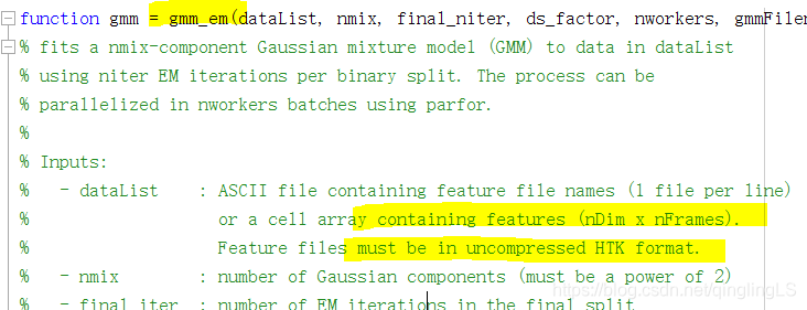
1. training a UBM from background data
(训练ubm通用背景模型,可以得知,这里的训练数据最好比较大,另外不要把特定人识别的训练数据也拿进去)
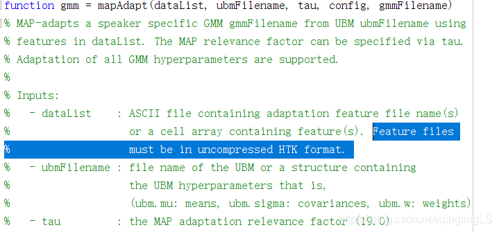
2. MAP adapting speaker models from the UBM using enrollment data
(在得到的有256个高斯元的混合高斯模型上,进行特定人的数据map,也就是求这些人在模型上的参数)
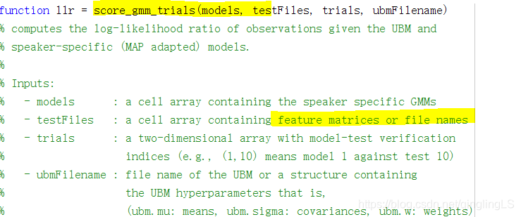
3. scoring verification trials
(给验证模型打分)
4. computing the performance measures (e.g., EER)
(计算性能表现测度,比如说err值)
有个类似的参考网址:
https://blog.youkuaiyun.com/u010592995/article/details/77340761
我用的是下面的代码:
clc
clear
%% Step0: Opening MATLAB pool 并行执行,记得关掉其他的大cpu占用应用
nworkers = 12; %理想的核数
nworkers = min(nworkers, feature('NumCores'));%你的电脑的cpu核数和理想核数取最小值
if isempty(gcp('nocreate'))
parpool;
end
%% Step1: Training the UBM 训练背景模型
dataList = 'lists/ubm.lst';
nmix = 256; %高斯核数,越大,拟合能力越强
final_niter = 10; %迭代次数
ds_factor = 1;
ubm = gmm_em(dataList, nmix, final_niter, ds_factor, 4);
save('ubm.mat','ubm') % load和save很必要,如果运行到某一段出现错误,可以直接加载上一段的 数据继续执行,不必从头开始
% ubm = load('ubm.mat')
% ubm = ubm.ubm
%% Step2: Adapting the speaker models from UBM 在UBM得到的模型上进行map
fea_dir = ''; %特征地址
fea_ext = ''; %特征拓展名
fid = fopen('lists/speaker_model_maps.lst', 'rt');
C = textscan(fid, '%s %s');
fclose(fid);
model_ids = unique(C{1}, 'stable');
model_files = C{2};
nspks = length(model_ids);
map_tau = 10.0;
config = 'mvw';
gmm_models = cell(nspks, 1);
for spk = 1 : nspks,
ids = find(ismember(C{1}, model_ids{spk}));
spk_files = model_files(ids);
spk_files = cellfun(@(x) fullfile(fea_dir, [x, fea_ext]),... %# Prepend path to files
spk_files, 'UniformOutput', false);
gmm_models{spk} = mapAdapt(spk_files, ubm, map_tau, config);
end
save('gmm_models.mat','gmm_models')
% gmm_models = load('gmm_models.mat')
% gmm_models = gmm_models.gmm_models
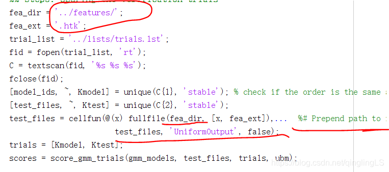
%% Step3: Scoring the verification trials 打分
fea_dir = '';
fea_ext = '';
trial_list = 'lists/trials.lst';
fid = fopen(trial_list, 'rt');
C = textscan(fid, '%s %s %s');
fclose(fid);
[model_ids, ~, Kmodel] = unique(C{1}, 'stable'); % check if the order is the same as above!
[test_files, ~, Ktest] = unique(C{2}, 'stable');
test_files = cellfun(@(x) fullfile(fea_dir, [x, fea_ext]),... %# Prepend path to files
test_files, 'UniformOutput', false);
trials = [Kmodel, Ktest];
scores = score_gmm_trials(gmm_models, test_files, trials, ubm);
save('scores.mat','scores')
% scores = load('scores.mat')
% scores = scores.scores
%% Step4: Computing the EER and plotting the DET curve
imagesc(reshape(scores,56*2, 39)) % 这里的56*2是每个模型的测试样本数量,39是模型数目,所以score的大小为4368
title('Speaker Verification Likelihood (GMM Model)');
ylabel('Test # (Channel x Speaker)'); xlabel('Model #');
colorbar;drawnow; axis xy
figure
labels = C{3};
eer = compute_eer(scores, labels, true);
涉及了三个表:
程序需要读取三个文件:ubm.lst、speaker_model_maps.lst、trials.lst
ubm.lst : 用来训练UBM,包含xx个人共xxx个特征文件路径名,格式为
特征路径名
speaker_model_maps.lst:用来适应训练人的特征路径名 格式为为
人名 特征路径名
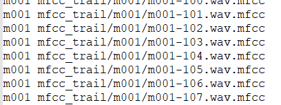
trials.lst : 每个模型(人名)都对应所有测试语句,格式为
人名 特征路径名 标签

第一列为人名,也即模型名,每个模型要对应100个测试语句,所以这个模型名的有100行,中间的为100个特征路径名,最后一列为标签,只有属于第一列模型的语句才是target,其它的都为imposter,
生成上面的三个表的脚本:
我使用了全部文件夹里的200-259号文件,
后面我把后39个人的行删掉了,那就是前117-39人的数据作为背景了,
记得删,(训练ubm通用背景模型,可以得知,这里的训练数据最好比较大,另外不要把特定人识别的训练数据也拿进去)
参考在timid数据集上的demo示例链接:
https://blog.youkuaiyun.com/u010592995/article/details/77340761
python:ubm.lst
#!/usr/bin/python
# -*- coding:utf8 -*-

import os

# 遍历指定目录,显示目录下的所有文件名
def eachFile(filepath,f):
    pathDir = os.listdir(filepath)
    for allDir in pathDir:
        child = os.path.join('%s%s' % (filepath, allDir))
        # child.decode('gbk')  # .decode('gbk')是解决中文显示乱码问题
        names=allDir.split("-")
        if os.path.isfile(child) and allDir[0]=='m':
            print(names)
            id=int(names[1].split(".")[0])
            if id>=200 and id<260:
                f.write(("mfcc_trail/"+names[0]+"/"+allDir+".mfcc\n").replace('D:\\说话人确认项目资源文件\\my-htk\\', ''))
        #f.write(child+" ")
        if(allDir[0]=='m' and os.path.isdir(child)):
            eachFile(child+"\\",f)

if __name__ == '__main__':
    f = open('D:\\说话人确认项目资源文件\\my-htk\\ubm.lst', 'w')
    filePath = "D:\\说话人确认项目资源文件\\my-htk\\Beijing\\"
    eachFile(filePath,f)
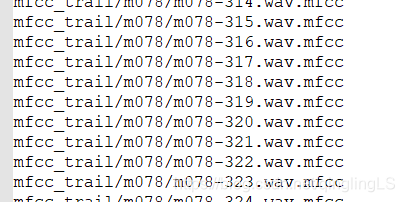
生成trails:
#!/usr/bin/python
# -*- coding:utf8 -*-

import os

# 遍历指定目录,显示目录下的所有文件名
def eachFile(filepath,f,parent_name):
    pathDir = os.listdir(filepath)
    t=0
    x=0
    for allDir in pathDir:
        child = os.path.join('%s%s' % (filepath, allDir))
        # child.decode('gbk')  # .decode('gbk')是解决中文显示乱码问题
        names=allDir.split("-")
        path=""
        if len(names)==2:
            id=int(names[1].split(".")[0])
            path=names[0]
            if path == parent_name and id>144 and t<=10:
                print("ture")
                f.write((parent_name + " mfcc_trail/" + parent_name + "/" + allDir + " target\n").replace(
                    'D:\\说话人确认项目资源文件\\my-htk\\', ''))
                t+=1
            elif path != parent_name and x<=100:
                f.write((parent_name + " mfcc_trail/" + parent_name + "/" + allDir + " impostor\n").replace(
                    'D:\\说话人确认项目资源文件\\my-htk\\', ''))
                x+=1

        print(allDir)
        if os.path.isfile(child) and allDir[0]=='m':
            print("")
            # f.write((names[0]+" mfcc_trail/"+names[0]+"/"+allDir+".mfcc impostor\n").replace('D:\\说话人确认项目资源文件\\my-htk\\', ''))
        #f.write(child+" ")
        if(allDir[0]=='m' and os.path.isdir(child)):
            eachFile(child+"\\",f,allDir)

if __name__ == '__main__':
    f = open('D:\\说话人确认项目资源文件\\my-htk\\trials.lst', 'w')
    filePath = "D:\\说话人确认项目资源文件\\my-htk\\code\\mfcc_trail\\"
    eachFile(filePath,f,"mfcc_trail")
生成speaker_model_maps.lst可以自己改下上面生成ubm的脚本得到。
下面给出我弄好的:
下载地址:https://download.youkuaiyun.com/download/qinglingls/11960023
数据集处理:
根据样例材料和现有数据,我设计的方案是117人,其中的前78个人每个人390个句子,每个人的200到260句作为背景,也就是7860=4680句话用于训练UBM,剩下的39个人用前143个句子进行训练,得到39个模型,测试句子有11239=4368句。样本112个,有11句真,101句假冒者
另外在原来的代码中,
这里用的是.htk文件格式,
前面的ubm模型是用特征系数mfcc做的,
后面的mapadapt要用未经过压缩的htk格式,
我看了半天的代码。
对于每一段语音(可以取10-20帧作为一段,也就是2410或2420的矩阵),用MAP算法得到每一段语音(比如说当前段为0.01秒~0.02秒)对应的GMM模型的参数(2.2.2节的2.14-2.22式),theta_i, 然后再计算下一段语音(下一段为0.02秒~0.03秒)对应的参数theta_j,
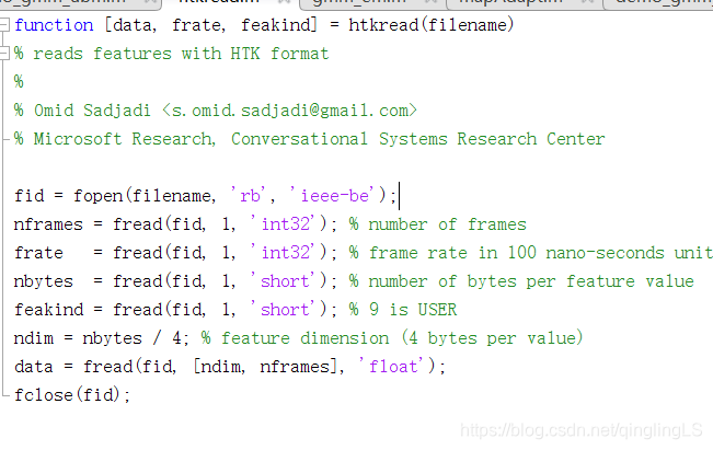
原始的音频数据文件(如WAV)转换成HTK格式的参数文件。
这里应指的就是mfcc特征文件啊!!!!(想到秃头!!!!)
所以为什么表述都不一样……??不懂了……
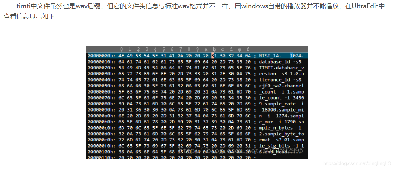
而在在 参考的timid数据集里面是它已经修改好文件头的文件了,并不能播放。
最后得到结果:
Initializing the GMM hyperparameters …
Re-estimating the GMM hyperparameters for 1 components …
EM iter#: 1 [llk = -88.31] [elaps = 1120.19 s]
Re-estimating the GMM hyperparameters for 2 components …
EM iter#: 2 [llk = -87.42] [elaps = 103.04 s]
Re-estimating the GMM hyperparameters for 4 components …
EM iter#: 4 [llk = -84.58] [elaps = 34.04 s]
Re-estimating the GMM hyperparameters for 8 components …
EM iter#: 4 [llk = -83.32] [elaps = 34.66 s]
Re-estimating the GMM hyperparameters for 16 components …
EM iter#: 4 [llk = -82.11] [elaps = 9.43 s]
Re-estimating the GMM hyperparameters for 32 components …
EM iter#: 4 [llk = -81.28] [elaps = 12.08 s]
Re-estimating the GMM hyperparameters for 64 components …
EM iter#: 6 [llk = -80.36] [elaps = 78.73 s]
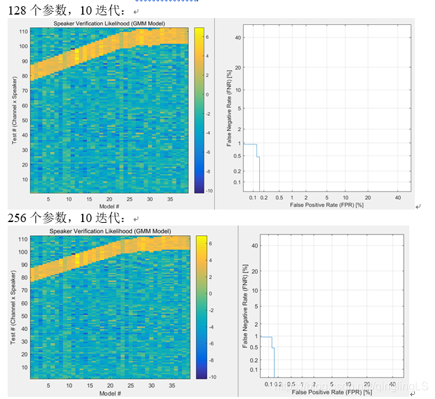
Re-estimating the GMM hyperparameters for 128 components …
EM iter#: 6 [llk = -79.59] [elaps = 57.55 s]
Re-estimating the GMM hyperparameters for 256 components …
EM iter#: 10 [llk = -78.68] [elaps = 50.00 s]
原错误率:50%
EER:0.372643577378343
FPR:
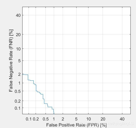
比较正常的数据应该是:
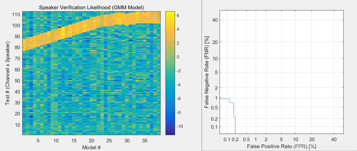
显示的相似度:
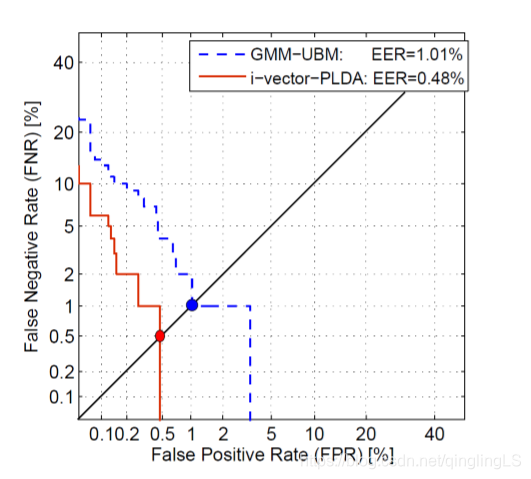
timid里面的结果:
出现上面的曲线的原因:
也许和数据有关,我的实验过程中效果很好。
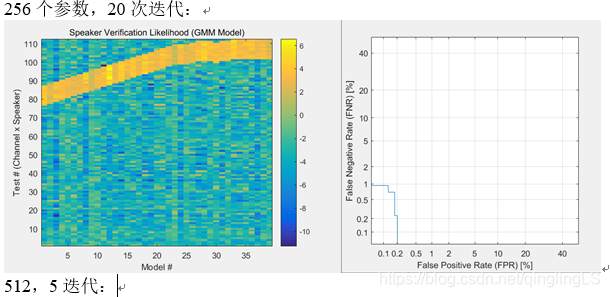
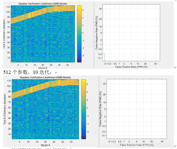
结论:
- 性能和判别器效果和模型大小有关,
模型表达能力很强时,少迭代次数也能达到很好的效果 - 性能和迭代次数相关,迭代次数增加,效果一定程度上变好,但是也要受到模型限制。
- 训练数据对训练过程起重要作用。
- 选择合适的模型时,比较少的样本就可以得出100%正确。实际中合理选择判断阈值,可以将FNR与FPR降到1%以下。


 1万+
1万+


 到【灌水乐园】发言


