PyTorch：nn模型层+nn方法

概述

torch.nn 中的模块是通过类的实例进行调用，通常需要先创建模型实例，再将输入数据传入模型中进行前向计算。

torch.nn.functional 中的函数可以直接调用，只需要将输入数据传入函数中即可进行前向计算。

编码

[onehot和multihot编码]

Embedding初始化及自定义

nn.Embedding

torch.nn.Embedding(num_embeddings: int, embedding_dim: int, padding_idx: Optional[int] = None, max_norm: Optional[float] = None, norm_type: float = 2.0, scale_grad_by_freq: bool = False, sparse: bool = False, _weight: Optional[torch.Tensor] = None)

参数

前面两个参数的简单理解：torch.nn.Embedding(m, n)。m 表示单词的总数目，n 表示词嵌入的维度，其实词嵌入就相当于是一个大矩阵，矩阵的每一行表示一个单词。

num_embeddings (int) – size of the dictionary of embeddings 词典的大小尺寸，比如总共出现5000个词，那就输入5000。此时index为（0-4999）。注意这里num_embeddings必须要比词对应的最大index要大，而不是比词个数大就可以。

embedding_dim (int) – the size of each embedding vector 嵌入向量的维度，即用多少维来表示一个符号。embedding_dim的选择要注意，根据自己的符号数量，举个例子，如果你的词典尺寸是1024，那么极限压缩（用二进制表示）也需要10维，再考虑词性之间的相关性，怎么也要在15-20维左右。

padding_idx (int, optional) – If given, pads the output with the embedding vector at padding_idx (initialized to zeros) whenever it encounters the index. 填充id，这样，网络在遇到填充id时，就不会计算其与其它符号的相关性（直接初始化为0）。

max_norm (float, optional) – If given, each embedding vector with norm larger than max_norm is renormalized to have norm max_norm.最大范数，如果嵌入向量的范数超过了这个界限，就要进行再归一化。

norm_type (float, optional) – The p of the p-norm to compute for the max_norm option. Default 2. 指定利用什么范数计算，并用于对比max_norm，默认为2范数。

scale_grad_by_freq (boolean, optional) – If given, this will scale gradients by the inverse of frequency of the words in the mini-batch. Default False.根据单词在mini-batch中出现的频率，对梯度进行放缩。默认为False。

sparse (bool, optional) – If True, gradient w.r.t. weight matrix will be a sparse tensor. See Notes for more details regarding sparse gradients.若为True,则与权重矩阵相关的梯度转变为稀疏张量。

_weight (Tensor) - 形状为(num_embeddings, embedding_dim)，模块中可学习的权值（初始化时的）。

变量

~Embedding.weight (Tensor) – the learnable weights of the module of shape (num_embeddings, embedding_dim) initialized from 

Embedding类有个属性weight，是torch.nn.parameter.Parameter类型，作用就是存储真正的word embeddings。如果不给weight赋值，Embedding类会自动给他初始化，看源码[SOURCE]可知如果属性weight没有手动赋值，则会定义一个torch.nn.parameter.Parameter对象，然后对该对象进行reset_parameters()，对self.weight先转为Tensor在对其进行normal_(0, 1)(调整为$N(0, 1)$正态分布)。所以nn.Embeddig.weight默认初始化方式就是N(0, 1)分布，即均值$\mu=0$，方差$\sigma=1$的标准正态分布。

[源代码解析][nn.Embedding.weight初始化分布]

设置

1 如果不需要更新embedding，可以使用self.embedding.weight.requires_grad = False

2 如果embedding初始化后想修改初始化

比如默认是(0,1)的正态分布初始化，改成(0, 0.1)

方法1：

for tensor in embedding_dict.values():
    nn.init.normal_(tensor.weight, mean=0, std=init_std)
    with torch.no_grad():    # <=> tensor.weight.data[PAD_ID].fill_(0) 
        tensor.weight[PAD_ID].fill_(0)  

方法2：

row_ids = list(range(0, 7))
row_ids.remove(padding_idx)
embedding.weight.data[row_ids, :].normal_(0, 0.1)

方法3：通过_weight参数（不推荐）。

nn.Embedding(vocab_size, embed_size, sparse=sparse, _weight=torch.normal(mean=0, std=init_std, size=(vocab_size, embed_size)))
Note: 当指定_weight时， padding_idx=PAD_ID是无效的，看源码就知道了。

emdedding初始化

默认是随机初始化。
# 定义词嵌入
embeds = nn.Embedding(2, 5)    # 2 个单词，维度 5
# 得到词嵌入矩阵,开始是随机初始化的
torch.manual_seed(1)
embeds.weight
#-0.8923 -0.0583 -0.1955 -0.9656  0.4224
# 0.2673 -0.4212 -0.5107 -1.5727 -0.1232
#[torch.FloatTensor of size 2x5]

embed提取

注意参数只能是LongTensor型的。

读取一个向量

# 访问第 50 个词的词向量，即取出第50行的数据。
embeds = nn.Embedding(100, 10)
embeds(Variable(torch.LongTensor([50])))
# 输出：
Variable containing:
 0.6353  1.0526  1.2452 -1.8745 -0.1069  0.1979  0.4298 -0.3652 -0.7078  0.2642
[torch.FloatTensor of size 1x10]

读取多个向量
输入为两个维度(batch的大小，每个batch的单词个数)，输出维度=两个维度加上词向量的维度。

Input: LongTensor (N, W), N = mini-batch, W = number of indices to extract per mini-batch
Output: (N, W, embedding_dim)

embedding = nn.Embedding(10, 3)
# 每批取两组，每组四个单词
input = Variable(torch.LongTensor([[1,2,4,5],[4,3,2,9]]))
a = embedding(input) # 输出2*4*3

[pytorch中的embedding词向量的使用]

示例

示例1

self.word_embeddings = nn.Embedding(config.vocab_size, config.hidden_dim, padding_idx=config.pad_idx)
self.position_embeddings = nn.Embedding(config.max_content_len, config.hidden_dim)

示例2

padding_idx = 0   # 一般padding字符对应的id的embedding要全是0，且不可学习
embedding = nn.Embedding(7, 5, padding_idx=padding_idx)

hello_idx = torch.tensor([[0, 2, 1], [5, 4, 6]])  # batch(2)*maxlen(3)
hello_embed = embedding(hello_idx)
print(hello_embed)

Bugfix

size mismatch for embedding_dict.char.weight: copying a param with shape torch.Size([2772, 20]) from checkpoint, the shape in current model is torch.Size([829, 20]).
原因：当前模型使用的数据word数为829个（可能通过lang文件初始化）；而checkpoint中load_stat的模型的embedding_dict记录的word数为2772个，说明lang文件和checkpoint没对齐，需要检查一下此时使用的lang文件和checkpoint文件是不是同一个模型训练出来的。

[torch.nn > Embedding]

[通俗讲解pytorch中nn.Embedding原理及使用]

linear层

​torch.nn.Linear​

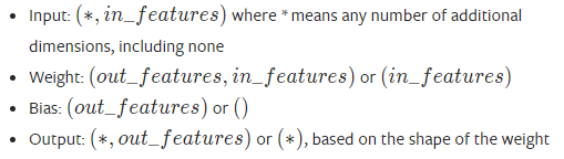
torch.nn.Linear(in_features, out_features, bias=True, device=None, dtype=None)

参数Parameters
        in_features (int) – size of each input sample

        out_features (int) – size of each output sample

        bias (bool) – If set to False, the layer will not learn an additive bias. Default: True

示例

m = nn.Linear(20, 30)
input = torch.randn(128, 20)
output = m(input)
print(output.size())

forward实际是通过return F.linear(input, self.weight, self.bias)实现

torch.nn.functional.linear​

torch.nn.functional.linear(input, weight, bias=None) 

Applies a linear transformation to the incoming data: y=input * weight^T + bias.

Shape:

nn.LayerNorm层归一化

nn.LayerNorm(normalized_shape, eps=1e-05, elementwise_affine=True, device=None, dtype=None)

示例

>>> input = torch.randn(20, 5, 10, 10)
>>> # With Learnable Parameters
>>> m = nn.LayerNorm(input.size()[1:])
>>> # Without Learnable Parameters
>>> m = nn.LayerNorm(input.size()[1:], elementwise_affine=False)
>>> # Normalize over last two dimensions 对最后2维进行LN，如一个句子的所有词的embedding
>>> m = nn.LayerNorm([10, 10])
>>> # Normalize over last dimension of size 10 对最后一维（比如embedding维度）进行LN
>>> m = nn.LayerNorm(10)
>>> # Activating the module
>>> output = m(input)

[LayerNorm]

padding填充

mask填充TENSOR.MASKED_FILL

Fills elements of self tensor with value where mask is True. 
示例：bert_output=(batch,seq_len,dim), mask=(batch,seq_len)
bert_output_masked = bert_output.masked_fill(mask=(mask == 0).unsqueeze(dim=2), value=0)

[torch.Tensor.masked_fill — PyTorch 2.0 documentation]

填充句子到相同长度nn.utils.rnn.pad_sequence

nn.utils.rnn.pad_sequence(sequences, batch_first=False, padding_value=0.0)

用padding_value 填充一系列可变长度的tensor，把它们填充到等长

示例1：

>>> from torch.nn.utils.rnn import pad_sequence
>>> a = torch.ones(25, 300)
>>> b = torch.ones(22, 300)
>>> c = torch.ones(15, 300)
>>> pad_sequence([a, b, c]).size()
torch.Size([25, 3, 300])

示例2：

from torch.nn.utils.rnn import pad_sequence
import torch
a=torch.randn(3)
b=torch.randn(5)
c=torch.randn(7)
>>> a
tensor([ 0.7160,  1.2006, -1.8447])
>>> b
tensor([ 0.3941,  0.3839,  0.1166, -0.7221,  1.8661])
>>> c
tensor([-0.6521,  0.0681,  0.6626, -0.3679, -0.6042,  1.6951,  0.4937])
>>> pad_sequence([a,b,c],batch_first=True,padding_value=1)
tensor([[ 0.7160,  1.2006, -1.8447,  1.0000,  1.0000,  1.0000,  1.0000],
        [ 0.3941,  0.3839,  0.1166, -0.7221,  1.8661,  1.0000,  1.0000],
        [-0.6521,  0.0681,  0.6626, -0.3679, -0.6042,  1.6951,  0.4937]])

[pad_sequence —— 填充句子到相同长度]

PADDED句子压缩NN.UTILS.RNN.PACK_PADDED_SEQUENCE

torch.nn.utils.rnn.pack_padded_sequence(input, lengths, batch_first=False,enforce_sorted=True)

参数
input：经过 pad_sequence 处理之后的数据。

lengths：mini-batch中各个序列的实际长度。

batch_first：True 对应 [batch_size, seq_len, feature]；False对应 [seq_len, batch_size, feature]。

enforce_sorted：如果是 True ，则输入应该是按长度降序排序的序列。如果是 False ，会在函数内部进行排序。默认值为 True 。

输出：

PackedSequence(data=tensor([1, 9, 2, 3, 4]),  batch_sizes=tensor([2, 1, 1, 1]), 
               sorted_indices=None, unsorted_indices=None)

pack 的意思可以理解为压紧或压缩 ，因为数据在经过填充之后，会有很多冗余的 padding_value，所以需要压缩一下。

mini-batch 中的 0 只是用来做数据对齐的 padding_value ，如果进行 forward 计算时，把 padding_value 也考虑进去，可能会导致RNN通过了非常多无用的 padding_value，这样不仅浪费计算资源，最后得到的值可能还会存在误差。

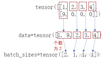
填充值 0 就被跳过了。PackedSequence数据结构中batch_size 的值，实际上就是告诉网络每个时间步需要吃进去多少数据。

示例1：先排序再pack_padded_sequence再过rnn再pad_packed_sequence再反排序

sorted_seq_lengths, indices = torch.sort(seq_lengths, descending=True)
sorted_inputs = inputs[:, indices]
packed_inputs = torch.nn.utils.rnn.pack_padded_sequence(sorted_inputs, sorted_seq_lengths.cpu(), batch_first=True)

outputs, state = self.rnn(packed_inputs, init_state)
pad_output, _ = torch.nn.utils.rnn.pad_packed_sequence(outputs, batch_first=True)

_, revert_indices = torch.sort(indices, descending=False)
pad_output = pad_output[revert_indices]

[rnn.py#L63]

示例2：在pack_padded_sequence内部排序

这个不建议，rnn输入未动，输出排序了，会对不齐。

packed_inputs = torch.nn.utils.rnn.pack_padded_sequence(inputs, seq_lengths.cpu(), batch_first=True, enforce_sorted=True)

压缩句子解压NN.UTILS.RNN.PAD_PACKED_SEQUENCE

[torch.nn.utils.rnn.pad_packed_sequence — PyTorch 2.0 documentation]

参数
sequences：PackedSequence 对象，将要被填充的 batch ；

batch_first：一般设置为 True，返回的数据格式为 [batch_size, seq_len, feature] ；

padding_value：填充值；

total_length：如果不是None，输出将被填充到长度：total_length。默认是None，代码中对应是max_seq_length。

如果在喂给网络数据的时候，用了 pack_sequence 进行打包，pytorch 的 RNN 也会把输出 out 打包成一个 PackedSequence 对象。

这个函数实际上是 pack_padded_sequence 函数的逆向操作，就是把压紧的序列再填充回来，方便后面计算。

[pack_padded_sequence 和 pad_packed_sequence - 知乎]

RNN类Encoder-RNN|LSTM|GRU

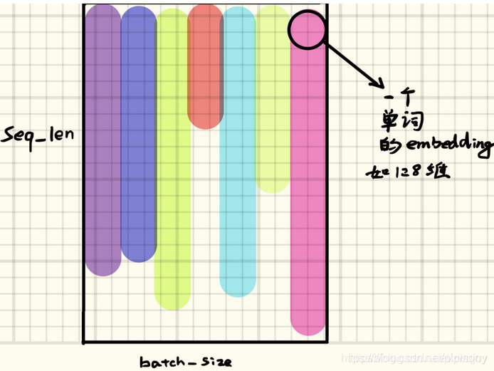
RNN 读取数据的方式：网络每次吃进去一组同样时间步 （time step） 的数据，也就是 mini-batch 的所有样本中下标相同的数据，然后获得一个 mini-batch 的输出；再移到下一个时间步 （time step），再读入 mini-batch 中所有该时间步的数据，再输出；直到处理完所有的时间步数据。

RNN

参数Parameters

input_size – The number of expected features in the input x

hidden_size – The number of features in the hidden state h

num_layers – Number of recurrent layers. E.g., setting num_layers=2 would mean stacking two RNNs together to form a stacked RNN, with the second RNN taking in outputs of the first RNN and computing the final results. Default: 1 堆叠层数

nonlinearity – The non-linearity to use. Can be either 'tanh' or 'relu'. Default: 'tanh'

bias – If False, then the layer does not use bias weights b_ih and b_hh. Default: True

batch_first – If True, then the input and output tensors are provided as (batch, seq, feature). Default: False. 注意，batch_first=True只是对input、output来说的，hidden层batch还是第二维。

dropout – If non-zero, introduces a Dropout layer on the outputs of each RNN layer except the last layer, with dropout probability equal to dropout. Default: 0

bidirectional – If True, becomes a bidirectional RNN. Default: False 是否使用双向rnn。

Note: RNN这里的序列长度，是动态的，不写在参数里的，具体会由输入的input参数而定。

Inputs: input, h_0
input维度 input of shape (seq_len, batch, input_size): tensor containing the features of the input sequence. The input can also be a packed variable length sequence. See torch.nn.utils.rnn.pack_padded_sequence() or torch.nn.utils.rnn.pack_sequence() for details.

h0维度 h_0 of shape (num_layers * num_directions, batch, hidden_size): tensor containing the initial hidden state for each element in the batch. Defaults to zero if not provided. If the RNN is bidirectional, num_directions should be 2, else it should be 1.h0是提供给每层RNN的初始输入，所有num_layers要和RNN的num_layers对得上。

Outputs: output, h_n
output of shape (seq_len, batch, num_directions * hidden_size): tensor containing the output features (h_t) from the last layer of the RNN, for each t. If a torch.nn.utils.rnn.PackedSequence has been given as the input, the output will also be a packed sequence.For the unpacked case, the directions can be separated using output.view(seq_len, batch, num_directions, hidden_size), with forward and backward being direction 0 and 1 respectively. Similarly, the directions can be separated in the packed case.RNN的上侧输出。

h_n of shape (num_layers * num_directions, batch, hidden_size): tensor containing the hidden state for t = seq_len.Like output, the layers can be separated using h_n.view(num_layers, num_directions, batch, hidden_size).RNN的右侧输出，如果是双向的话，就还有一个左侧输出。

具体参数和返回结果参考[RNN — PyTorch 2.0 documentation]

示例

rnn=nn.RNN(10,20,2) #(each_input_size, hidden_state, num_layers)
input=torch.randn(5,3,10) # (seq_len, batch, input_size)
h0=torch.randn(2,3,20) #(num_layers * num_directions, batch, hidden_size)
output,hn=rnn(input,h0)
print(output.size(),hn.size())

LSTM

[LSTM — PyTorch 2.0 documentation]

输出：

        output保存了最后一层每个time step的输出h（横向），如果是双向LSTM，每个time step的输出h = [h正向, h逆向] (同一个time step的正向和逆向的h连接起来)。(L,N,D∗Hout​) when batch_first=False or (N,L,D∗Hout​) when batch_first=True 。

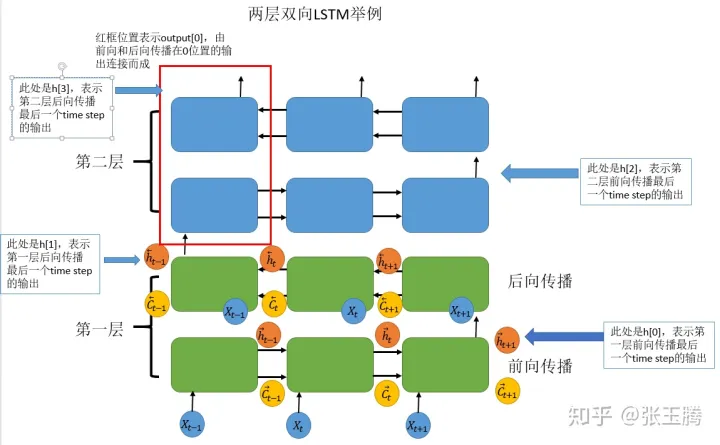
        h_n保存了每一层最后一个time step的输出h（纵向），如果是双向LSTM，单独保存前向和后向的最后一个time step的输出h（也就是说h_i保存的是中间或最后过程中要输出到下一步的decoder_state）。containing the final hidden state for each element in the sequence. When bidirectional=True, h_n will contain a concatenation of the final forward and reverse hidden states, respectively. (D∗num_layers,N,Hout)

        c_n与h_n一致，只是它保存的是c的值。c_n:  containing the final cell state for each element in the sequence.

Note: 如果单层单向lstm输入一个(batch_size, seq=1, hidden_dim)的向量，那output.squeeze(dim=1)和h_n.squeeze(dim=0)应该一样。

[聊一聊PyTorch中LSTM的输出格式 - 知乎]

示例1：

lstm = nn.LSTM(input_size=4, hidden_size=4, num_layers=1, # dropout=0.1,
               batch_first=True, bidirectional=True)
input = torch.randn(3, 5, 4)  # (batch, seq_len, input_size)
output, (hn, cn) = lstm(input)
print(output.size(), hn.size(), cn.size())

# output: batch x seq_len x hidden*bi_directional
# torch.Size([3, 5, 8]) torch.Size([2, 3, 4]) torch.Size([2, 3, 4])

示例2：

rnn = nn.LSTM(10, 20, 2)  # (each_input_size, hidden_state, num_layers)
input = torch.randn(5, 3, 10)  # (seq_len, batch, input_size)
h0 = torch.randn(2, 3, 20)  # (num_layers * num_directions, batch, hidden_size)
c0 = torch.randn(2, 3, 20)  # (num_layers * num_directions, batch, hidden_size)
output, (hn, cn) = rnn(input, (h0, c0))  # output: seq_len x batch x hidden*bi_directional
print(output.size(), hn.size(), cn.size())
# torch.Size([5, 3, 20]) torch.Size([2, 3, 20]) torch.Size([2, 3, 20])

示例3：

取最后一层的hn
last_layers_hn = h_n[D * (num_layers - 1):]

GRU

torch.nn.GRU(self, input_size, hidden_size, num_layers=1, bias=True, batch_first=False, dropout=0.0, bidirectional=False, device=None, dtype=None)

示例

import torch

rnn = torch.nn.GRU(input_size=2, hidden_size=4, num_layers=3, bidirectional=True, batch_first=True)
input = torch.randn(3, 5, 2)  # (batch, seq, input_size)
# h0 = torch.randn(2 * 3, 3, 4)
h0 = None
output, hn = rnn(input, h0)
print(output.size(), hn.size())
# torch.Size([3, 5, 8]) torch.Size([6, 3, 4])    # (batch, seq, hidden_size*D), (num_layers*D, batch, hidden_size)

卷积/padding/pooling api

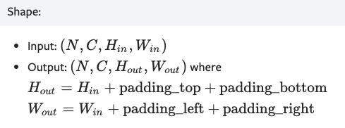
填充ConstantPad2d

torch.nn.ConstantPad2d(padding: Union[T, Tuple[T, T, T, T]], value: float)

参数：padding (int, tuple) – the size of the padding. If is int, uses the same padding in all boundaries. If a 4-tuple, uses padding_left , padding_right , padding_top , padding_bottom )

示例：

>>> m = nn.ConstantPad2d(2, 3.5)
>>> input = torch.randn(1, 2, 2)
>>> input
tensor([[[ 1.6585,  0.4320],
         [-0.8701, -0.4649]]])
>>> m(input)
tensor([[[ 3.5000,  3.5000,  3.5000,  3.5000,  3.5000,  3.5000],
         [ 3.5000,  3.5000,  3.5000,  3.5000,  3.5000,  3.5000],
         [ 3.5000,  3.5000,  1.6585,  0.4320,  3.5000,  3.5000],
         [ 3.5000,  3.5000, -0.8701, -0.4649,  3.5000,  3.5000],
         [ 3.5000,  3.5000,  3.5000,  3.5000,  3.5000,  3.5000],
         [ 3.5000,  3.5000,  3.5000,  3.5000,  3.5000,  3.5000]]])
>>> # using different paddings for different sides
>>> m = nn.ConstantPad2d((3, 0, 2, 1), 3.5)
>>> m(input)
tensor([[[ 3.5000,  3.5000,  3.5000,  3.5000,  3.5000],
         [ 3.5000,  3.5000,  3.5000,  3.5000,  3.5000],
         [ 3.5000,  3.5000,  3.5000,  1.6585,  0.4320],
         [ 3.5000,  3.5000,  3.5000, -0.8701, -0.4649],
         [ 3.5000,  3.5000,  3.5000,  3.5000,  3.5000]]])

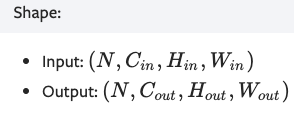
二维巻积CONV2D

torch.nn.Conv2d(in_channels: int, out_channels: int, kernel_size: Union[T, Tuple[T, T]], stride: Union[T, Tuple[T, T]] = 1, padding: Union[T, Tuple[T, T]] = 0, dilation: Union[T, Tuple[T, T]] = 1, groups: int = 1, bias: bool = True, padding_mode: str = 'zeros')

参数：in_channels：输入通道数。一般第1层是1个通道，如果是多层cnn堆叠，从第二层起通道数为上层的输出feature maps数=即上一层的out_channels。

Note:每层参数量计算。第l层参数量：C_in*C_out*kernel_size[l][0]*kernel_size[l][1]，其中C_in即in_channels[l]。

示例：

>>> # With square kernels and equal stride
>>> m = nn.Conv2d(16, 33, 3, stride=2)

Conv2d(1, 8, kernel_size=[3, 3], stride=(1, 1))

Conv2d(8, 16, kernel_size=[3, 3], stride=(1, 1))

自适应池化Adaptive Pooling

torch.nn.AdaptiveAvgPool2d(output_size: Union[T, Tuple[T, ...]])

普通Max/AvgPooling计算公式为：output_size = ceil ( (input_size+2∗padding−kernel_size)/stride）+1 

当我们使用Adaptive Pooling时，这个问题就变成了由已知量input_size，output_size求解kernel_size与stride。你只需要告诉torch你需要什么样的输出结果。

为了简化问题，我们将padding设为0（后面我们可以发现源码里也是这样操作的c++源码部分）

stride = floor ( (input_size / (output_size) )

kernel_size = input_size − (output_size−1) * stride

padding = 0

示例：

>>> # target output size of 5x7
>>> m = nn.AdaptiveAvgPool2d((5,7))
>>> input = torch.randn(1, 64, 8, 9)
>>> output = m(input)

>>> # target output size of 7x7 (square)
>>> m = nn.AdaptiveAvgPool2d(7)
>>> input = torch.randn(1, 64, 10, 9)
>>> output = m(input)

[[开发技巧]·AdaptivePooling与Max/AvgPooling相互转换]

一维巻积CONV1D

torch.nn.Conv1d(in_channels, out_channels, kernel_size, stride=1, padding=0, dilation=1, groups=1, bias=True, padding_mode='zeros')

in_channels(int) – 输入信号的通道。在文本分类中，即为词向量的维度
out_channels(int) – 卷积产生的通道。有多少个out_channels，就需要多少个1维卷积
kernel_size(int or tuple) - 卷积核的尺寸，卷积核的大小为(k,)，第二个维度是由in_channels来决定的，所以实际上卷积大小为kernel_size*in_channels
stride(int or tuple, optional) - 卷积步长
padding (int or tuple, optional)- 输入的每一条边补充0的层数
dilation(int or tuple, `optional``) – 卷积核元素之间的间距
groups(int, optional) – 从输入通道到输出通道的阻塞连接数
bias(bool, optional) - 如果bias=True，添加偏置

示例

常用于textcnn[深度学习：文本CNN-textcnn]

conv1 = nn.Conv1d(in_channels=256，out_channels=100,kernel_size=2)
input = torch.randn(32,35,256)
# batch_size x text_len x embedding_size -> batch_size x embedding_size x text_len
input = input.permute(0,2,1)
out = conv1(input)
print(out.size())

这里32为batch_size，35为句子最大长度，256为词向量。在输入一维卷积的时候，需要将32*35*256变换为32*256*35，因为一维卷积是在最后维度上扫的，最后out的大小即为：32*100*（35-2+1）=32*100*34。

[pytorch之nn.Conv1d详解]

from: -柚子皮-

ref: