


 本文深入讲解逻辑回归算法,包括其原理、Sigmoid函数、损失函数、梯度下降法及代码实现,通过鸢尾花数据集演示分类预测,探讨决策边界绘制与过拟合处理。
逻辑回归——(Logistic Regression)
1-是什么?
逻辑回归是一种解决分类问题的算法(尤其是二分类问题)。
2-如何解决分类问题?
将样本的特征和样本的发生的概率联系起来。
对于一个样本 x x x ,我们通过函数 f f f 求得其发生的概率 p ^ = f ( x ) \hat{p} = f(x) p^=f(x)
若
p
^
=
{
1
,
i
f
p
^
≥
0.5
0
,
i
f
p
^
<
0.5
\hat{p} = \begin{cases} 1, & if& \hat{p} \ge 0.5\\ 0, & if& \hat{p} \lt 0.5 \end{cases}
p^={1,0,ififp^≥0.5p^<0.5
在线性回归问题中,我们通过寻找一组最佳拟合训练样本的参数
θ
\theta
θ ,使得对于任意一个预测样本
X
b
X_b
Xb ,其预测值可通过
y
^
=
θ
T
⋅
X
b
\hat{y} = {\theta}^T·X_b
y^=θT⋅Xb 来求得。然而这样求得的结果,其值域处于
(
−
∞
,
+
∞
)
(-\infty,+\infty)
(−∞,+∞) ,我们如何才能将这一结果约束到
[
0
,
1
]
[0,1]
[0,1] 这个范围呢?
3-Sigmoid函数
Sigmoid函数的表达形式为:
σ
(
t
)
=
1
1
+
e
−
t
\sigma(t) = \frac{1}{1+e^{-t}}
σ(t)=1+e−t1
其函数图像为:
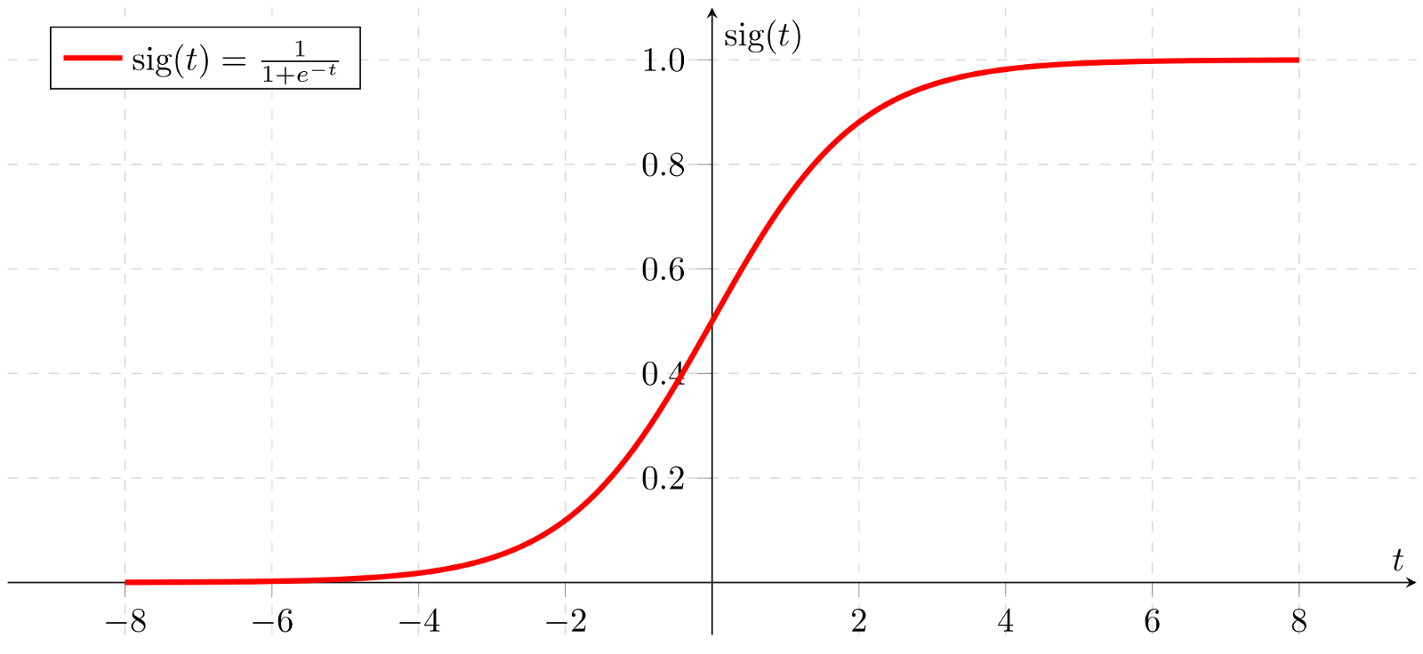
这样我们就可以通过Sigmoid函数讲预测值 y ^ \hat{y} y^ 约束在 [ 0 , 1 ] [0,1] [0,1] 这个范围内了。
4-Cost Function
我们如何确定一个损失函数,从而寻找到一组最佳的 θ \theta θ 来拟合我们的训练数据呢?显然我们要寻找的损失函数必须满足一下条件:
设:一个给定样本其发生的概率为
p
^
\hat{p}
p^
C
o
s
t
=
{
如
果
y
=
1
,
p
^
越
小
,
c
o
s
t
越
大
如
果
y
=
0
,
p
^
越
大
,
c
o
s
t
越
大
Cost=\begin{cases} 如果y=1,\hat{p}越小,cost越大\\ 如果y=0,\hat{p}越大,cost越大 \end{cases}
Cost={如果y=1,p^越小,cost越大如果y=0,p^越大,cost越大
因此如下函数可以满足上述要求:
C
o
s
t
=
{
−
l
o
g
(
p
^
)
i
f
y
=
1
−
l
o
g
(
1
−
p
^
)
i
f
y
=
0
Cost = \begin{cases} -log(\hat{p}) & if&y=1\\ -log(1-\hat{p}) & if&y=0 \end{cases}
Cost={−log(p^)−log(1−p^)ifify=1y=0
进一步我们可以讲上述分段函数合并:
C
o
s
t
=
−
y
l
o
g
(
p
^
)
−
(
1
−
y
)
l
o
g
(
1
−
p
^
)
Cost = -ylog(\hat{p})-(1-y)log(1-\hat{p})
Cost=−ylog(p^)−(1−y)log(1−p^)
对于目标函数
J
(
θ
)
J(\theta)
J(θ) 有:
J
(
θ
)
=
−
1
m
∑
i
=
1
m
[
y
(
i
)
l
o
g
(
p
^
(
i
)
)
+
(
1
−
y
(
i
)
)
l
o
g
(
1
−
p
^
(
i
)
)
]
J(\theta)=-\frac{1}{m} \sum_{i=1}^{m}\lbrack y^{(i)}log({\hat{p}^{(i)}})+(1-y^{(i)})log(1-{\hat{p}}^{(i)})\rbrack
J(θ)=−m1i=1∑m[y(i)log(p^(i))+(1−y(i))log(1−p^(i))]
其中:
p
^
(
i
)
=
σ
(
X
b
(
i
)
⋅
θ
)
=
1
1
+
e
−
X
b
(
i
)
θ
\hat{p}^{(i)}=\sigma(X_b^{(i)}·\theta)=\frac{1}{1+e^{-X_b^{(i)}\theta}}
p^(i)=σ(Xb(i)⋅θ)=1+e−Xb(i)θ1
将
p
^
(
i
)
\hat{p}^{(i)}
p^(i) 带入到
J
(
θ
)
J(\theta)
J(θ) 中得:
J
(
θ
)
=
−
1
m
∑
i
=
1
m
[
y
(
i
)
l
o
g
(
1
1
+
e
−
X
b
(
i
)
θ
)
+
(
1
−
y
(
i
)
)
l
o
g
(
1
−
1
1
+
e
−
X
b
(
i
)
θ
)
]
J(\theta) =-\frac{1}{m} \sum_{i=1}^{m}\lbrack y^{(i)}log({\frac{1}{1+e^{-X_b^{(i)}\theta}}})+(1-y^{(i)})log(1-{\frac{1}{1+e^{-X_b^{(i)}\theta}}})\rbrack
J(θ)=−m1i=1∑m[y(i)log(1+e−Xb(i)θ1)+(1−y(i))log(1−1+e−Xb(i)θ1)]
至此,我们接下来需要解决的问题就是求目标函数
J
(
θ
)
J(\theta)
J(θ) 的最小值了,而这个最小值并不能通过数学推到得出,而需要我们运用前面所学习的梯度下降算法来求出。
5-目标函数的梯度求解(数学推导)
在求解梯度之前我们先整理一下我们的目标函数:
J
(
θ
)
=
−
1
m
∑
i
=
1
m
[
y
(
i
)
l
o
g
(
σ
(
t
)
)
+
(
1
−
y
(
i
)
)
l
o
g
(
1
−
σ
(
t
)
)
]
J(\theta)=-\frac{1}{m} \sum_{i=1}^{m}\lbrack y^{(i)}log({\sigma(t)})+(1-y^{(i)})log(1-\sigma(t))\rbrack
J(θ)=−m1i=1∑m[y(i)log(σ(t))+(1−y(i))log(1−σ(t))]
这里我们将
p
^
(
i
)
\hat{p}^{(i)}
p^(i) 改写为了
σ
(
t
)
\sigma(t)
σ(t) 使得式子看起来更简洁一点,便于我们稍候的处理。
首先我们来求
σ
(
t
)
=
(
1
+
e
−
t
)
−
1
\sigma(t)=(1+e^{-t})^{-1}
σ(t)=(1+e−t)−1 的倒数
σ
′
(
t
)
=
−
(
1
+
e
−
t
)
−
2
⋅
e
−
t
⋅
(
−
1
)
=
e
−
t
(
1
+
e
−
t
)
2
\sigma^{'}(t) =-(1+e^{-t})^{-2}·e^{-t}·(-1) =\frac{e^{-t}}{(1+e^{-t})^2}
σ′(t)=−(1+e−t)−2⋅e−t⋅(−1)=(1+e−t)2e−t
对于
l
o
g
[
σ
(
t
)
]
log\lbrack\sigma(t)\rbrack
log[σ(t)] 求导:
l
o
g
[
σ
(
t
)
]
′
=
1
σ
(
t
)
⋅
σ
′
(
t
)
=
1
σ
(
t
)
⋅
e
−
t
(
1
+
e
−
t
)
2
=
1
(
1
+
e
−
t
)
−
1
⋅
e
−
t
(
1
+
e
−
t
)
2
=
e
−
t
(
1
+
e
−
t
)
{log\lbrack\sigma(t)\rbrack}^{'} =\frac{1}{\sigma(t)}·\sigma^{'}(t)\\ =\frac{1}{\sigma(t)}·\frac{e^{-t}}{(1+e^{-t})^2} = \frac{1}{(1+e^{-t})^{-1}}·\frac{e^{-t}}{(1+e^{-t})^2} = \frac{e^{-t}}{(1+e^{-t})}
log[σ(t)]′=σ(t)1⋅σ′(t)=σ(t)1⋅(1+e−t)2e−t=(1+e−t)−11⋅(1+e−t)2e−t=(1+e−t)e−t
在这里我们做一个简单的变换,在
e
−
t
(
1
+
e
−
t
)
\frac{e^{-t}}{(1+e^{-t})}
(1+e−t)e−t 的分子上
+
1
+1
+1 再
−
1
-1
−1 :
l
o
g
[
σ
(
t
)
]
′
=
1
+
e
−
t
−
1
(
1
+
e
−
t
)
=
1
−
1
1
+
e
−
t
=
1
−
σ
(
t
)
{log\lbrack\sigma(t)\rbrack}^{'} =\frac{1+e^{-t}-1}{(1+e^{-t})}=1-\frac{1}{1+e^{-t}}=1-\sigma(t)
log[σ(t)]′=(1+e−t)1+e−t−1=1−1+e−t1=1−σ(t)
同样的我们再求
l
o
g
[
1
−
σ
(
t
)
]
log\lbrack1-\sigma(t)\rbrack
log[1−σ(t)] 的倒数:
l
o
g
[
1
−
σ
(
t
)
]
′
=
1
1
−
σ
(
t
)
⋅
(
−
1
)
⋅
σ
(
t
)
′
=
−
1
1
−
σ
(
t
)
⋅
(
1
+
e
−
t
)
−
2
⋅
e
−
t
{log\lbrack 1-\sigma(t) \rbrack}^{'}=\frac{1}{1-\sigma(t)}·(-1)·{\sigma(t)}^{'} =-\frac{1}{1-\sigma(t)}·(1+e^{-t})^{-2}·e^{-t}
log[1−σ(t)]′=1−σ(t)1⋅(−1)⋅σ(t)′=−1−σ(t)1⋅(1+e−t)−2⋅e−t
其中
−
1
1
−
σ
(
t
)
=
1
1
+
e
−
t
1
+
e
−
t
−
1
1
+
e
−
t
=
−
1
+
e
−
t
e
−
t
-\frac{1}{1-\sigma(t)} = \frac{1}{{\frac{1+e^{-t}}{1+e^{-t}}}-\frac{1}{1+e^{-t}}} = -\frac{1+e^{-t}}{e^{-t}}
−1−σ(t)1=1+e−t1+e−t−1+e−t11=−e−t1+e−t
带入上式:
l
o
g
[
1
−
σ
(
t
)
]
′
=
−
1
+
e
−
t
e
−
t
⋅
(
1
+
e
−
t
)
−
2
⋅
e
−
t
=
−
1
1
+
e
−
t
=
−
σ
(
t
)
{log\lbrack 1-\sigma(t)\rbrack}^{'} =-\frac{1+e^{-t}}{e^{-t}}·(1+e^{-t})^{-2}·e^{-t} =-\frac{1}{1+e^{-t}}=-\sigma(t)
log[1−σ(t)]′=−e−t1+e−t⋅(1+e−t)−2⋅e−t=−1+e−t1=−σ(t)
我们知道
θ
\theta
θ 是一个
n
n
n 维列向量,其表达形式可以表示为:
θ
=
[
θ
1
,
θ
2
,
…
,
θ
j
−
1
,
,
θ
j
,
θ
j
+
1
,
…
,
,
θ
n
]
T
\theta = [{\theta}_1,{\theta}_2,\dots,{\theta}_{j-1},,{\theta}_j,{\theta}_{j+1},\dots,,{\theta}_n]^T
θ=[θ1,θ2,…,θj−1,,θj,θj+1,…,,θn]T
我们求
J
(
θ
)
J(\theta)
J(θ) 在
θ
j
{\theta}_j
θj 方向上的倒数:
d
[
J
(
θ
)
]
d
θ
j
=
−
1
m
∑
i
=
1
m
y
(
i
)
[
1
−
σ
(
X
b
(
i
)
⋅
θ
)
]
⋅
X
j
(
i
)
+
(
1
−
y
(
i
)
)
⋅
[
−
σ
(
X
b
(
i
)
⋅
θ
)
]
⋅
X
j
(
i
)
\frac{d\lbrack J(\theta)\rbrack}{d{\theta}_j} = -\frac{1}{m}\sum_{i=1}^{m}y^{(i)}\lbrack1-\sigma({X_b}^{(i)}·\theta)\rbrack·{X_j}^{(i)}+(1-y^{(i)})·\lbrack-\sigma({X_b}^{(i)}·\theta)\rbrack·{X_j}^{(i)}
dθjd[J(θ)]=−m1i=1∑my(i)[1−σ(Xb(i)⋅θ)]⋅Xj(i)+(1−y(i))⋅[−σ(Xb(i)⋅θ)]⋅Xj(i)
=
−
1
m
∑
i
=
1
m
y
(
i
)
⋅
X
j
(
i
)
−
y
(
i
)
σ
(
X
b
(
i
)
⋅
θ
)
⋅
X
j
(
i
)
−
σ
(
X
b
(
i
)
⋅
θ
)
⋅
X
j
(
i
)
+
y
(
i
)
σ
(
X
b
(
i
)
⋅
θ
)
⋅
X
j
(
i
)
= -\frac{1}{m}\sum_{i=1}^{m}y^{(i)}·{X_j}^{(i)}-y^{(i)}\sigma({X_b}^{(i)}·\theta)·{X_j}^{(i)}-\sigma({X_b}^{(i)}·\theta)·{X_j}^{(i)}+y^{(i)}\sigma({X_b}^{(i)}·\theta)·{X_j}^{(i)}
=−m1i=1∑my(i)⋅Xj(i)−y(i)σ(Xb(i)⋅θ)⋅Xj(i)−σ(Xb(i)⋅θ)⋅Xj(i)+y(i)σ(Xb(i)⋅θ)⋅Xj(i)
=
1
m
∑
i
=
1
m
[
σ
(
X
b
(
i
)
⋅
θ
)
−
y
(
i
)
]
⋅
X
j
(
i
)
= \frac{1}{m}\sum_{i=1}^{m}\lbrack \sigma({X_b}^{(i)}·\theta)-y^{(i)} \rbrack·{X_j}^{(i)}
=m1i=1∑m[σ(Xb(i)⋅θ)−y(i)]⋅Xj(i)
对于
J
(
θ
)
J(\theta)
J(θ) 我们在
θ
j
{\theta}_j
θj 方向上求导是如此,对于其他方向上的求导亦是如此。
故
J
(
θ
)
J(\theta)
J(θ) 在
θ
\theta
θ 方向上的梯度
∇
J
(
θ
)
=
(
∂
J
∂
θ
0
∂
J
∂
θ
1
⋮
∂
J
∂
θ
n
)
=
1
m
(
∑
i
=
1
n
(
σ
(
X
b
(
i
)
⋅
θ
)
)
−
y
(
i
)
∑
i
=
1
n
[
(
σ
(
X
b
(
i
)
⋅
θ
)
)
−
y
(
i
)
]
⋅
X
1
(
i
)
⋮
∑
i
=
1
n
[
(
σ
(
X
b
(
i
)
⋅
θ
)
)
−
y
(
i
)
]
⋅
X
n
(
i
)
)
\nabla J(\theta) = {\begin{pmatrix} \frac{\partial J}{\partial {\theta}_0}\\ \frac{\partial J}{\partial {\theta}_1}\\ \vdots\\ \frac{\partial J}{\partial {\theta}_n}\\ \end{pmatrix}} =\frac{1}{m}\begin{pmatrix} \sum_{i=1}^{n}(\sigma({X_b}^{(i)}·\theta))-y^{(i)}\\ \sum_{i=1}^{n}\lbrack(\sigma({X_b}^{(i)}·\theta))-y^{(i)}\rbrack·{X_1}^{(i)}\\ \vdots\\ \sum_{i=1}^{n}\lbrack(\sigma({X_b}^{(i)}·\theta))-y^{(i)}\rbrack·{X_n}^{(i)}\\ \end{pmatrix}
∇J(θ)=⎝⎜⎜⎜⎛∂θ0∂J∂θ1∂J⋮∂θn∂J⎠⎟⎟⎟⎞=m1⎝⎜⎜⎜⎛∑i=1n(σ(Xb(i)⋅θ))−y(i)∑i=1n[(σ(Xb(i)⋅θ))−y(i)]⋅X1(i)⋮∑i=1n[(σ(Xb(i)⋅θ))−y(i)]⋅Xn(i)⎠⎟⎟⎟⎞
回忆我们在学习现行回归是对梯度结果进行向量化的过程
∇
J
(
θ
)
=
2
m
⋅
(
∑
i
=
1
m
(
X
b
(
i
)
⋅
θ
−
y
(
i
)
)
∑
i
=
1
m
(
X
b
(
i
)
⋅
θ
−
y
(
i
)
)
⋅
X
1
(
i
)
∑
i
=
1
m
(
X
b
(
i
)
⋅
θ
−
y
(
i
)
)
⋅
X
2
(
i
)
⋮
∑
i
=
1
m
(
X
b
(
i
)
⋅
θ
−
y
(
i
)
)
⋅
X
n
(
i
)
)
=
2
m
⋅
X
b
T
⋅
(
X
b
θ
−
y
)
\nabla J(\theta) = \frac{2}{m}· \begin{pmatrix} \sum_{i=1}^m({X_b}^{(i)}·\theta-y^{(i)})\\ \sum_{i=1}^m({X_b}^{(i)}·\theta-y^{(i)})·{X_1}^{(i)}\\ \sum_{i=1}^m({X_b}^{(i)}·\theta-y^{(i)})·{X_2}^{(i)}\\ \vdots \\ \sum_{i=1}^m({X_b}^{(i)}·\theta-y^{(i)})·{X_n}^{(i)}\\ \end{pmatrix} =\frac{2}{m}·{X_b}^T·(X_b\theta-y)
∇J(θ)=m2⋅⎝⎜⎜⎜⎜⎜⎜⎛∑i=1m(Xb(i)⋅θ−y(i))∑i=1m(Xb(i)⋅θ−y(i))⋅X1(i)∑i=1m(Xb(i)⋅θ−y(i))⋅X2(i)⋮∑i=1m(Xb(i)⋅θ−y(i))⋅Xn(i)⎠⎟⎟⎟⎟⎟⎟⎞=m2⋅XbT⋅(Xbθ−y)
因此我们同样可以讲我们计算的梯度进行向量化运算,最后得到的结果就是:
∇
J
(
θ
)
=
1
m
⋅
X
b
T
⋅
[
σ
(
X
b
⋅
θ
)
−
y
]
\nabla J(\theta) = \frac{1}{m}·{X_b}^T·\lbrack \sigma(X_b·\theta)-y \rbrack
∇J(θ)=m1⋅XbT⋅[σ(Xb⋅θ)−y]
6-代码实现
我们封装了一个类,在这个类中可以进行fit、predict 等操作,具体代码如下
import numpy as np
class LogisticRegression:
    def __init__(self):
        """初始化LogisticRegression模型"""
        self.coef_ = None
        self.interception_ = None
        self._theta = None
    def _sigmoid(self,t):
        return 1./(1. + np.exp(-t))
    def fit(self,X_train,y_train,eta=0.01,n_iterations=1e4):
        """根据训练数据集X_train训练 Logistic Regression模型"""
        assert X_train.shape[0] == y_train.shape[0], \
            "the size of X_train must be equal to the size of y_train"
        def J(theta, X_b, y):
            y_hat = self._sigmoid(X_b.dot(theta))
            try:
                return - np.sum(y * np.log(y_hat) + (1 - y) * np.log(1 - y_hat)) / len(y)
            except:
                return float('inf')
        def dJ(theta, X_b, y):
            return X_b.T.dot(self._sigmoid(X_b.dot(theta)) - y) / len(X_b)
        def gradient_descent(X_b, y, initial_theta, eta, n_iterations=1e4, epsilon=1e-8):
            theta = initial_theta
            cur_iter = 0
            while cur_iter < n_iterations:
                gradient = dJ(theta,X_b,y)
                last_theta = theta
                theta = theta - eta * gradient
                if(abs(J(theta,X_b,y) - J(last_theta,X_b,y)) < epsilon):
                    break
                cur_iter +=1
            return theta
        X_b = np.hstack([np.ones((len(X_train), 1)), X_train])
        initial_theta = np.zeros(X_b.shape[1])
        self._theta = gradient_descent(X_b,y_train,initial_theta,eta,n_iterations)
        self.interception_ = self._theta[0]
        self.coef_ = self._theta[1:]
    def predict_proba(self, X_predict):
        """给定待测数据集 X_predict,返回X_predict的结果概率向量"""
        assert self.interception_ is not None and self.coef_ is not None, \
            "must fit berore predict"
        assert X_predict.shape[1] == len(self.coef_), \
            "the feature number of X_predict must be equal to X_train"
        X_b = np.hstack([np.ones((len(X_predict), 1)), X_predict])
        return self._sigmoid(X_b.dot(self._theta))
    def predict(self, X_predict):
        """给定待测数据集 X_predict,返回X_predict的结果向量"""
        assert self.interception_ is not None and self.coef_ is not None,\
            "must fit berore predict"
        assert X_predict.shape[1] == len(self.coef_),\
            "the feature number of X_predict must be equal to X_train"
        proba = self.predict_proba(X_predict)
        return np.array(proba >= 0.5, dtype='int')
    def score(self, X_test, y_test):
        """根据测试数据集 X_test 和 y_test 确定当前模型的精确度"""
        y_predict = self.predict(X_test)
        return sum(y_predict == y_test)/len(y_test)
    def __repr__(self):
        return "LogisticRegression()"
下面我们使用sklearn 中的 datasets 导入鸢尾花数据集来检验我们封装的方法是否正确
import numpy as np
import matplotlib.pyplot as plt
from sklearn import datasets
iris = datasets.load_iris()
X = iris.data
y = iris.target
X = X[y < 2, :2]
y = y[y < 2]
plt.scatter(X[y == 0, 0], X[y == 0, 1], color="red")
plt.scatter(X[y == 1, 0], X[y == 1, 1], color="blue")
plt.show()

在这里我们对鸢尾花的数据作了一部分筛除,因为逻辑回归适用于二分类问题,所以我们使用y<2 这样的操作来获得分类标签的前两个(Iris-Setosa和Iris-Versicolour),同样的我们也只取iris数据集中的前两个特征(sepal length 和 sepal width)
iris数据集包含下面四个特征
- sepal length in cm
- sepal width in cm
- petal length in cm
- petal width in cm
iris数据集包含下面三个分类
- Iris-Setosa
- Iris-Versicolour
- Iris-Virginica
下面我们从PlayML中导入封装的LogisticRegression和model_selection
from PlayML.model_selection import train_test_split
X_train, X_test, y_train, y_test = train_test_split(X, y, seed=666)
from PlayML.LogisticRegression import LogisticRegression
log_reg = LogisticRegression()
log_reg.fit(X_train, y_train)
log_reg.score(X_test, y_test)
输出结果为:
1.0
显然我们的模型百分之百地拟合了所有的测试数据,我们使用log_reg.predict_proba(X_test)来看看使用测试数据集预测得到的概率向量
array([0.92972035, 0.98664939, 0.14852024, 0.17601199, 0.0369836 ,
       0.0186637 , 0.04936918, 0.99669244, 0.97993941, 0.74524655,
       0.04473194, 0.00339285, 0.26131273, 0.0369836 , 0.84192923,
       0.79892262, 0.82890209, 0.32358166, 0.06535323, 0.20735334])
对比我们的y_test
array([1, 1, 0, 0, 0, 0, 0, 1, 1, 1, 0, 0, 0, 0, 1, 1, 1, 0, 0, 0])
不难发现,对于返回概率大于0.5的样本我们都标记为了1,对于小于0.5的样本我们都标记为了0;
7-决策边界
文章的开头我们知道逻辑回归的基本思想就是对于一个未知样本
X
b
X_{b}
Xb ,其分类标签
y
^
\hat{y}
y^
y
^
=
{
1
,
i
f
p
^
≥
0.5
0
,
i
f
p
^
<
0.5
\hat{y} = \begin{cases} 1, & if& \hat{p} \ge 0.5\\ 0, & if& \hat{p} \lt 0.5 \end{cases}
y^={1,0,ififp^≥0.5p^<0.5
其中
p
^
=
σ
(
X
b
⋅
θ
)
\hat{p}=\sigma(X_b·\theta)
p^=σ(Xb⋅θ)
我们通过观察Sigmoid函数的函数图像发现,当
{
X
b
⋅
θ
>
0
时
p
^
>
0.5
X
b
⋅
θ
<
0
时
p
^
<
0.5
\begin{cases} X_{b}·\theta>0 & 时 & \hat{p}>0.5\\ X_{b}·\theta<0 & 时 & \hat{p}<0.5 \end{cases}
{Xb⋅θ>0Xb⋅θ<0时时p^>0.5p^<0.5
因此有
y
^
=
{
1
,
i
f
X
b
⋅
θ
≥
0
0
,
i
f
X
b
⋅
θ
<
0
\hat{y} = \begin{cases} 1, & if& X_{b}·\theta \ge 0\\ 0, & if& X_{b}·\theta \lt 0 \end{cases}
y^={1,0,ififXb⋅θ≥0Xb⋅θ<0
显然当
X
b
⋅
θ
=
0
X_{b}·\theta=0
Xb⋅θ=0 的时候为决策边界,当
X
X
X 为二维时
X
b
⋅
θ
=
θ
0
+
θ
1
⋅
x
1
+
θ
2
⋅
x
2
X_b·\theta = {\theta}_0 +{\theta}_1·x_1 + {\theta}_2·x_2
Xb⋅θ=θ0+θ1⋅x1+θ2⋅x2
令其得零,则有
θ
0
+
θ
1
⋅
x
1
+
θ
2
⋅
x
2
=
0
{\theta}_0 +{\theta}_1·x_1 + {\theta}_2·x_2=0
θ0+θ1⋅x1+θ2⋅x2=0
θ
2
⋅
x
2
=
−
θ
0
−
θ
1
⋅
x
1
{\theta}_2·x_2=-{\theta}_0-{\theta}_1·x_1
θ2⋅x2=−θ0−θ1⋅x1
x
2
=
−
θ
0
−
θ
1
⋅
x
1
θ
2
x_2=\frac{-{\theta}_0-{\theta}_1·x_1}{{\theta}_2}
x2=θ2−θ0−θ1⋅x1
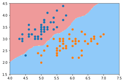
我们使用matplot画出这一决策边界
def x2(x1):
    return (-log_reg.coef_[0] * x1 - log_reg.interception_)/log_reg.coef_[1]
plt.scatter(X[y == 0, 0], X[y == 0, 1], color="red")
plt.scatter(X[y == 1, 0], X[y == 1, 1], color="blue")
x1_plot = np.linspace(4,8,1000)
x2_plot = x2(x1_plot)
plt.plot(x1_plot,x2_plot)
plt.show()
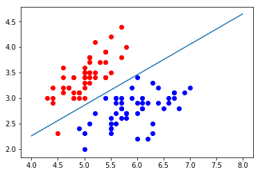
图中的直线就是所求的决策边界,能够很好地将两个分类分开,然而不知道您有没有注意到,在直线的下方蓝色点集中区域有一颗红点。这显然是一个错误分类,但是我们在代码实现的时候得到的正确率明明是 1.0 怎么会出现错误分类呢?这是因为我们的散点图是以训练数据集来绘制的,而我们在计算正确率的时候,使用的是测试数据集。
如果我们使用测试数据集来绘制散点图
def x2(x1):
    return (-log_reg.coef_[0] * x1 - log_reg.interception_)/log_reg.coef_[1]
plt.scatter(X_test[y_test == 0, 0], X_test[y_test == 0, 1], color="red")
plt.scatter(X_test[y_test == 1, 0], X_test[y_test == 1, 1], color="blue")
x1_plot = np.linspace(4,8,1000)
x2_plot = x2(x1_plot)
plt.plot(x1_plot,x2_plot)
plt.show()
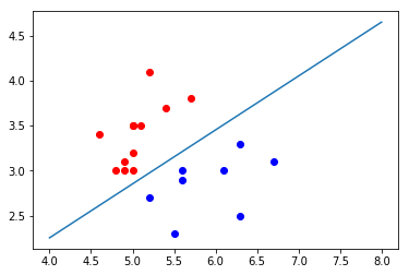
这样就与我们之前的计算精确度结果为1.0完全符合了
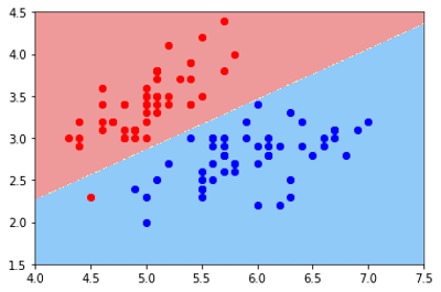
8-不规则决策边界的绘制
对于一个不规则的决策边界的绘制我们采用的方法是将平面划分为足够密的网格,然后对网格上所有的交叉点来判断它的分类,这样就可以近似的画出所要求的决策平面

下面我们就用代码来绘制我们在7中的决策边界吧
def plot_decision_boundary(model, axis):
    x0, x1 = np.meshgrid(
        np.linspace(axis[0], axis[1], int((axis[1]-axis[0])*100)).reshape(-1,1),
        np.linspace(axis[2], axis[3], int((axis[3]-axis[2])*100)).reshape(-1,1)
    )
    X_new = np.c_[x0.ravel(), x1.ravel()]
    y_predict = model.predict(X_new)
    zz = y_predict.reshape(x0.shape)
    from matplotlib.colors import ListedColormap
    custom_cmap = ListedColormap(['#EF9A9A','#FFF59D','#90CAF9'])
    plt.contourf(x0, x1, zz, cmap=custom_cmap)
plot_decision_boundary(log_reg,axis=[4,7.5,1.5,4.5])
plt.scatter(X[y == 0, 0], X[y == 0, 1], color="red")
plt.scatter(X[y == 1, 0], X[y == 1, 1], color="blue")
plt.show()
8-1 KNN的决策边界
我们使用KNN算法对上述鸢尾花数据进行预测,并绘制出决策边界
from sklearn.neighbors import KNeighborsClassifier
knn_clf = KNeighborsClassifier()
knn_clf.fit(X_train, y_train)
knn_clf.score(X_test, y_test)
plot_decision_boundary(knn_clf, axis=[4, 7.5, 1.5, 4.5])
plt.scatter(X[y==0,0], X[y==0,1])
plt.scatter(X[y==1,0], X[y==1,1])
plt.show()
在逻辑回归于上面的KNN例子中我们只对iris数据的两个标签进行了分类(Iris-Setosa和Iris-Versicolour),但是KNN是支持多标签分类的,所以我们现在对鸢尾花数据的三个标签进行分类并绘制出决策边界
knn_clf_all = KNeighborsClassifier()
knn_clf_all.fit(iris.data[:,:2], iris.target)
plot_decision_boundary(knn_clf_all, axis=[4, 8, 1.5, 4.5])
plt.scatter(iris.data[iris.target==0,0], iris.data[iris.target==0,1])
plt.scatter(iris.data[iris.target==1,0], iris.data[iris.target==1,1])
plt.scatter(iris.data[iris.target==2,0], iris.data[iris.target==2,1])
plt.show()
我们可以看到这样绘制的边界十分的不规则,这显然就是过拟合的表现,我们看一下此时KNN算法的参数n_neighbors的值等于多少
knn_clf_all.n_neighbors
Out:5
此时的n_neighbors=5当我们改变KNN算法中n_neighbors的参数为50时,看看结果会如何
knn_clf_all = KNeighborsClassifier(n_neighbors=50)
knn_clf_all.fit(iris.data[:,:2], iris.target)
plot_decision_boundary(knn_clf_all, axis=[4, 8, 1.5, 4.5])
plt.scatter(iris.data[iris.target==0,0], iris.data[iris.target==0,1])
plt.scatter(iris.data[iris.target==1,0], iris.data[iris.target==1,1])
plt.scatter(iris.data[iris.target==2,0], iris.data[iris.target==2,1])
plt.show()

可以看到此时的边界就平滑很多了
9-在逻辑回归中使用多项式特征
以上提到的鸢尾花数据都是线性可分的,那么对于线性不可分的数据我们如何使用逻辑回归来处理呢?下面看这样一个例子:
import numpy as np
import matplotlib.pyplot as plt
np.random.seed(666)
X = np.random.normal(0,1,size = (200,2))
y = np.array(X[:,0]**2 + X[:,1]**2 <1.5,dtype='int')
plt.scatter(X[y==0,0],X[y==0,1])
plt.scatter(X[y==1,0],X[y==1,1])
plt.show()
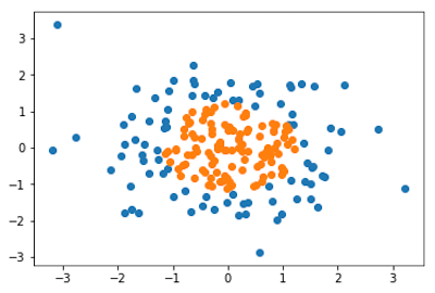
手动生成的数据,对于
{
x
0
2
+
x
1
2
≥
1.5
蓝
色
x
0
2
+
x
1
2
<
1.5
橙
色
\begin{cases} {x_0}^2+{x_1}^2 \ge 1.5 & 蓝色\\ {x_0}^2+{x_1}^2 \lt 1.5 & 橙色 \end{cases}
{x02+x12≥1.5x02+x12<1.5蓝色橙色
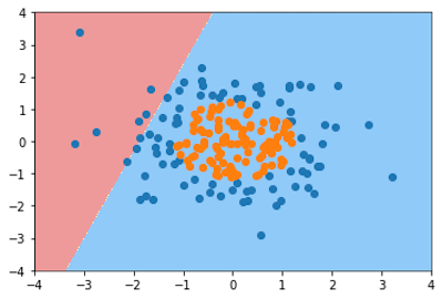
我们如果直接使用逻辑回归来处理
from PlayML.LogisticRegression import LogisticRegression
log_reg = LogisticRegression()
log_reg.fit(X,y)
log_reg.score(X,y)
Out:0.605
可以看到这个正确率显然是非常低的,我们再尝试绘制一下决策边界
def plot_decision_boundary(model, axis):
    x0, x1 = np.meshgrid(
        np.linspace(axis[0], axis[1], int((axis[1]-axis[0])*100)).reshape(-1,1),
        np.linspace(axis[2], axis[3], int((axis[3]-axis[2])*100)).reshape(-1,1)
    )
    X_new = np.c_[x0.ravel(), x1.ravel()]
    y_predict = model.predict(X_new)
    zz = y_predict.reshape(x0.shape)
    from matplotlib.colors import ListedColormap
    custom_cmap = ListedColormap(['#EF9A9A','#FFF59D','#90CAF9'])
    plt.contourf(x0, x1, zz, cmap=custom_cmap)
plot_decision_boundary(log_reg,axis=[-4,4,-4,4])
plt.scatter(X[y==0,0],X[y==0,1])
plt.scatter(X[y==1,0],X[y==1,1])
plt.show()
可以看到这里有非常多的错误分类,下面我们就为我们的逻辑回归添加多项式项来优化我们的逻辑回归算法(这里没有做训练测试数据切分,train_test_split)
from sklearn.pipeline import Pipeline
from sklearn.preprocessing import PolynomialFeatures
from sklearn.preprocessing import StandardScaler
def PolynomialLogisticRegression(degree):
    return Pipeline([
        ('poly', PolynomialFeatures(degree=degree)),
        ('std_scaler', StandardScaler()),
        ('log_reg', LogisticRegression())
    ])
poly_log_reg = PolynomialLogisticRegression(degree=2)
poly_log_reg.fit(X, y)
plot_decision_boundary(poly_log_reg, [-4, 4, -4, 4])
plt.scatter(X[y==0,0], X[y==0,1])
plt.scatter(X[y==1,0], X[y==1,1])
plt.show()
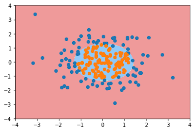
接下来看一下这个模型的准确度
poly_log_reg.score(X,y)
Out:0.95
可以看到准确度已经明显上升,而且数据也被很好好地拟合了。
如果我们再将参数degree调高一点会发生什么呢?
poly_log_reg2 = PolynomialLogisticRegression(degree=20)
poly_log_reg2.fit(X, y)
plot_decision_boundary(poly_log_reg2, [-4, 4, -4, 4])
plt.scatter(X[y==0,0], X[y==0,1])
plt.scatter(X[y==1,0], X[y==1,1])
plt.show()
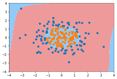
这里我们将参数degree调到了20,显然又发生了过拟合现象


 1907
1907

 被折叠的 条评论
为什么被折叠?
被折叠的 条评论
为什么被折叠?
 到【灌水乐园】发言


