CS224W摘要08.Applications of Graph Neural Networks

CS224W: Machine Learning with Graphs
公式输入请参考： 在线Latex公式
这节课要讲如何对图做augmentation
之前的讨论都是根据原始的图数据进行计算的，也就是说之前都是根据以下假设进行的：
Raw input graph = computational graph
但是实际上这个假设有很多问题：

1. Features:
   § The input graph lacks features
2. Graph structure:
   § The graph is too sparse →inefficient message passing
   § The graph is too dense →message passing is too costly（某些微博节点关注量上百万，做aggregation计算量太大）
   § The graph is too large →cannot fit the computational graph into a GPU

因此原始数据不一定适用直接进行计算，要对原始的图数据进行增强（处理）。
针对上面的两个方面问题，这节课也从两个方面进行讲解如何做增强。
Graph Feature augmentation
Graph Structure augmentation
§ The graph is too sparse →Add virtual nodes / edges
§ The graph is too dense →Sample neighbors when doing message passing
§ The graph is too large →Sample subgraphs to compute embeddings

Graph Feature augmentation

原因：
1.节点没有feature，只有结构信息（邻接矩阵）
解决方案：
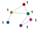
a）Assign constant values to nodes

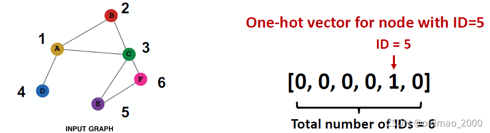
b）Assign unique IDs to nodes，一般使用独热编码

两个方案的对比如下表：

	方案a	方案b
Expressive power	Medium. All the nodes are identical, but GNN can still learn from the graph structure	High. Each node has a unique ID, so node-specific information can be stored
Inductive learning (Generalize to unseen nodes)	High. Simple to generalize to new nodes: we assign constant feature to them, then apply our GNN	Low. Cannot generalize to new nodes: new nodes introduce new IDs, GNN doesn’t know how to embed unseen IDs
Computational cost	Low. Only 1 dimensional feature	High. O（V） dimensional feature, cannot apply to large graphs
Use cases	Any graph, inductive settings (generalize to new nodes)	Small graph, transductive settings (no new nodes)

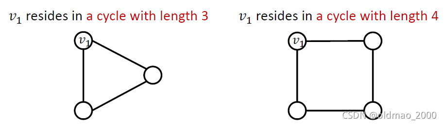
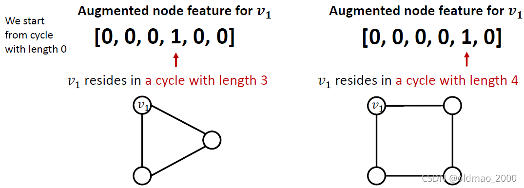
2.有些图结构GNN很难学习到，例如：Cycle count feature

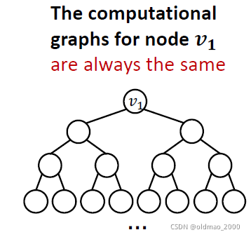
两个图中的$v_1$节点度都为2，以$v_1$节点做出来的计算图都是一样的二叉树

解决方案是把cycle count直接作为特征加到节点信息里面

当然还可以有别的特征可以加进来，例如：
§ Node degree
§ Clustering coefficient
§ PageRank
§ Centrality

Graph Structure augmentation

Augment sparse graphs

Add virtual edges

Connect 2-hop neighbors via virtual edges
该法与计算图的邻接矩阵：$A+A^2$效果一样
例如：Author-to-papers的Bipartite graph中

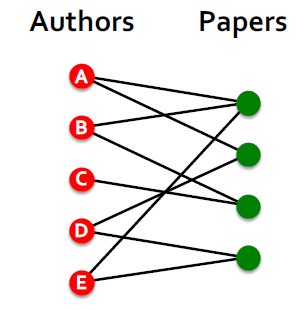
2-hop virtual edges make an author-author collaboration graph.

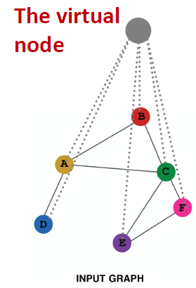
Add virtual nodes

The virtual node will connect to all the nodes in the graph.
§ Suppose in a sparse graph, two nodes have shortest path distance of 10.
§ After adding the virtual node, all the nodes will have a distance of two.
好处：
Greatly improves message passing in sparse graphs.

Augment dense graphs

方法就是对邻居节点进行采样操作。
例如，设置采样窗口大小为2，那么

可能变成：

当然，采样是随机的，所有还有可能是：

当然，如果邻居节点个数小于采样窗口大小，汇聚后的embedding会比较相似。
这个做法的好处是大大减少计算量。

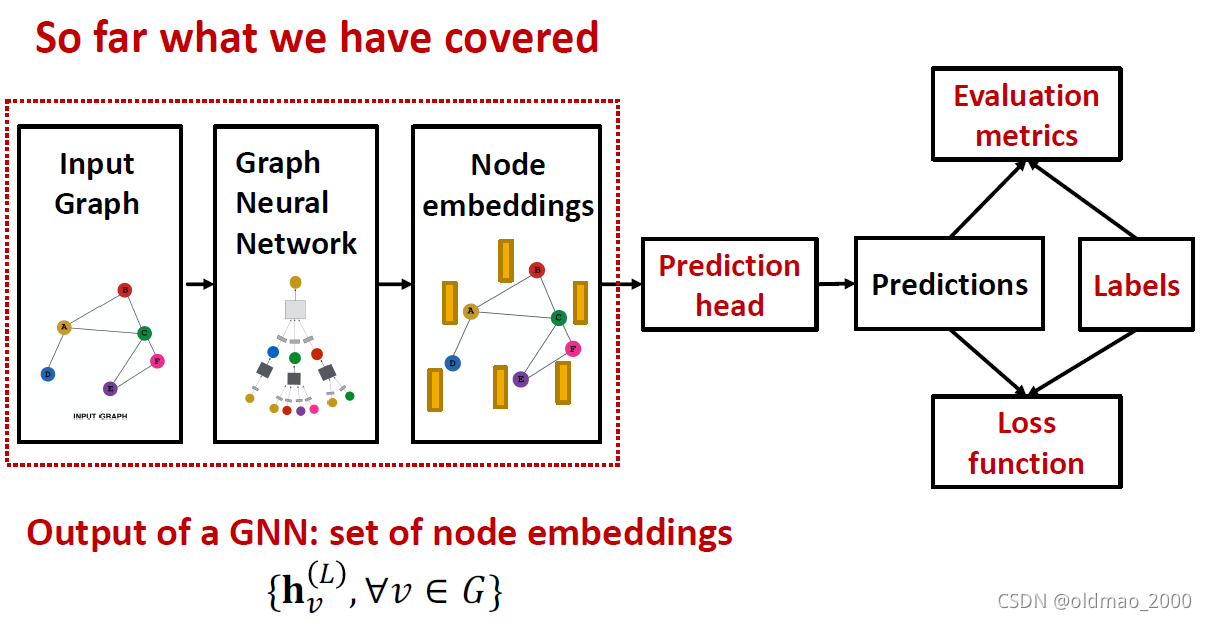
Prediction with GNNs

这个小节讲解GNN框架的预测部分：

GNN Prediction Heads

Idea: Different task levels require different prediction heads
这里第一次看到用Head来代表函数

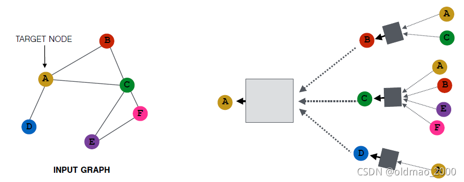
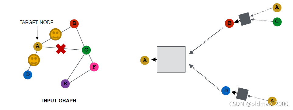
Node-level prediction

直接用节点表征进行预测
Suppose we want to make 𝑘-way prediction
§ Classification: classify among 𝑘 categories
§ Regression: regress on 𝑘 targets

$${\hat{y}}_v=Hea{d}_{node}{h}_v^{(L)}=W^{(H)}{h}_v^{(L)}$$

Edge-level prediction

用一对节点的表征对边进行预测：
$${\hat{y}}_{uv}=Hea{d}_{edge}(h_u^{(L)},h_v^{(L)})$$
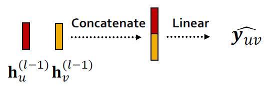
这里的Head有两种做法：
1.Concatenation + Linear

$${\hat{y}}_{uv}=Linear(Concat(h_u^{(L)},h_v^{(L)}))$$
这里的Linear操作会将2×d维的concat结果映射为 k-dim embeddings（相当于𝑘-way prediction）
2.Dot product
$${\hat{y}}_{uv}=(h_u^{(L)}{)}^T{h}_v^{(L)}$$
由于点积后得到的是常量，因此该方法用于𝟏-way prediction，通常是指边是否存在。
如果要把这个方法用在𝒌-way prediction，则可以参考多头注意力机制设置k个可训练的参数：$W^{(1)},W^{(2)},\cdots ,W^{(k)}$
$$\begin{gathered} {\hat{y}}_{uv}^{(1)}=(h_u^{(L)}{)}^T{W}^{(1)}{h}_v^{(L)} \\ \cdots \\ {\hat{y}}_{uv}^{(k)}=(h_u^{(L)}{)}^T{W}^{(k)}{h}_v^{(L)} \end{gathered}$$
$${\hat{y}}_{uv}=Concat(y_{uv}^{(1)},\cdots ,y_{uv}^{(k)})$$

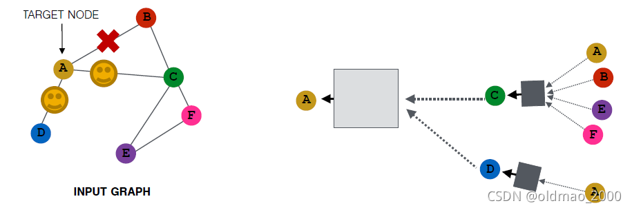
Graph-level prediction

使用图中所有节点的特征做预测。
y ^ G = H e a d g r a p h ( { h v ( L ) ∈ R d , ∀ v ∈ G } ) \hat y_G=Head_{graph}(\{h_v^{(L)}\in \R^d,\forall v\in G\}) y^​G​=Headgraph​({hv(L)​∈Rd,∀v∈G})
这里的head函数和aggregation操作很像，也是有mean、max、sum操作。
这些常规操作对于小图效果不错，对于大图效果不好，会掉信息。
例子：
we use 1-dim node embeddings
§ Node embeddings for 𝐺 1 : { − 1 , − 2 , 0 , 1 , 2 } 𝐺_1: \{−1,−2, 0, 1, 2\} G1​:{−1,−2,0,1,2}
§ Node embeddings for 𝐺 2 : { − 10 , − 20 , 0 , 10 , 20 } 𝐺_2: \{−10,−20, 0, 10, 20\} G2​:{−10,−20,0,10,20}
如果用sum做图的预测，上面两个图结果都是0，但是明显两个图是不一样的。

解决方案：
将所有节点的aggregation操作变hierarchically。
还是上面的例子，我们使用ReLU(Sum(⋅))作为head函数。然后分别把前面两个节点和后面3个节点分开做aggregation，最后再合并得到最后的预测结果。
第一轮：
G 1 : y ^ a = R e L U ( S u m ( { − 1 , − 2 } ) ) = 0 , y ^ b = R e L U ( S u m ( { 0 , 1 , 2 } ) ) = 3 G_1:\hat y_a=ReLU(Sum(\{-1,-2\}))=0,\hat y_b=ReLU(Sum(\{0,1,2\}))=3 G1​:y^​a​=ReLU(Sum({−1,−2}))=0,y^​b​=ReLU(Sum({0,1,2}))=3
G 2 : y ^ a = R e L U ( S u m ( { − 1 , − 2 } ) ) = 0 , y ^ b = R e L U ( S u m ( { 0 , 1 , 2 } ) ) = 30 G_2:\hat y_a=ReLU(Sum(\{-1,-2\}))=0,\hat y_b=ReLU(Sum(\{0,1,2\}))=30 G2​:y^​a​=ReLU(Sum({−1,−2}))=0,y^​b​=ReLU(Sum({0,1,2}))=30
第二轮：
G 1 : y ^ G 1 = R e L U ( S u m ( { y a , y b } ) ) = 3 G_1:\hat y_{G_1}=ReLU(Sum(\{y_a,y_b\}))=3 G1​:y^​G1​​=ReLU(Sum({ya​,yb​}))=3
G 2 : y ^ G 2 = R e L U ( S u m ( { y a , y b } ) ) = 30 G_2:\hat y_{G_2}=ReLU(Sum(\{y_a,y_b\}))=30 G2​:y^​G2​​=ReLU(Sum({ya​,yb​}))=30

由此可以得到DiffPool算法：

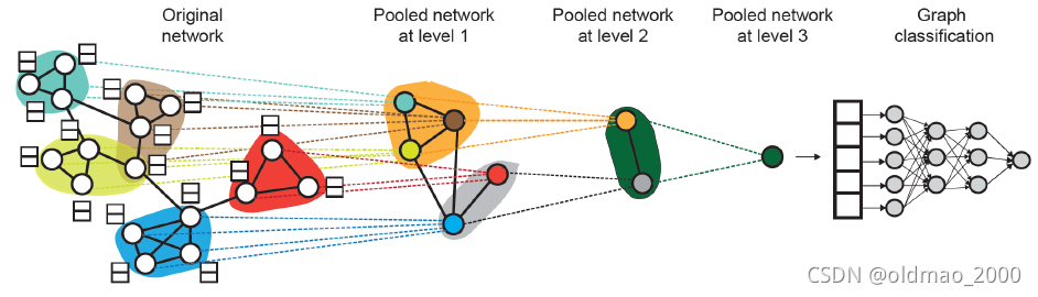
Leverage 2 independent GNNs at each level
§ GNN A: Compute node embeddings
§ GNN B: Compute the cluster that a node belongs to
A和B在每个level可以并行计算。

For each Pooling layer
§ Use clustering assignments from GNN B to aggregate node embeddings generated by GNN A
§ Create a single new node for each cluster, maintaining edges between clusters to generated a new pooled network
Jointly train GNN A and GNN B

Training Graph Neural Networks

这节主要是接着讲如何将预测结果和Label进行对比（Loss function）和评估（Evaluation metrics）。

Supervised vs Unsupervised

Supervised learning on graphs: Labels come from external sources
E.g., predict drug likeness of a molecular graph
Unsupervised learning on graphs: Signals come from graphs themselves
E.g., link prediction: predict if two nodes are connected
注意：Sometimes the differences are blurry

	Unsupervised	Supervised
Node labels ${\mathbf{y}}_{\mathbf{v}}$	Node statistics: such as clustering coefficient, PageRank, …	in a citation network, which subject area does a node belong to
Edgelabels ${\mathbf{y}}_{uv}$	Link prediction: hide the edge between two nodes, predict if there should be a link	in a transaction network, whether an edge is fraudulent
Graphlabels ${\mathbf{y}}_G$	Graph statistics: for example, predict if two graphs are isomorphic	among molecular graphs, the drug likeness of graphs

Loss

基础知识
We will use prediction ${\hat{y}}^{(i)}$, label $y^{(i)}$ to refer predictions at all levels(node/edge/graph)
分类或者回归不同在于loss function & evaluation metrics

Classification loss

labels $y^{(i)}$ with discrete value
E.g., Node classification: which category does a node belong to
As discussed in lecture 6, cross entropy (CE) is a very common loss function in classification
𝐾-way prediction for 𝑖-th data point:

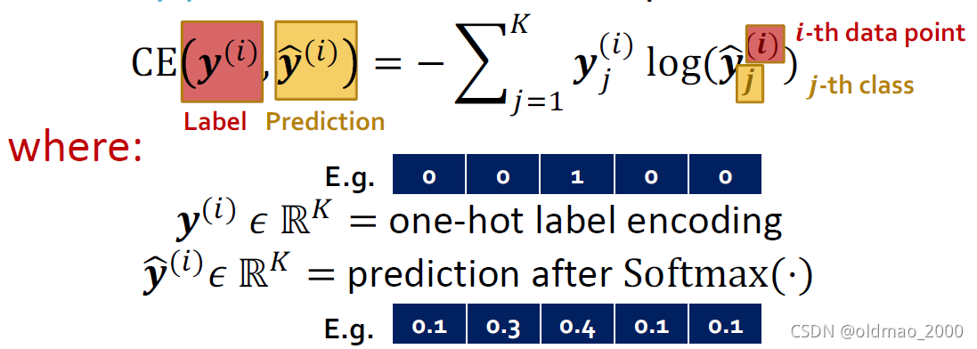
对于N个样本点，总的loss为：
$$Loss=\sum _{i=1}^{N}CE(y^{(i)},{\hat{y}}^{(i)})$$

Regression loss

labels $y^{(i)}$ with continuous value
E.g., predict the drug likeness of a molecular graph

For regression tasks we often use Mean Squared Error (MSE) a.k.a. L2 loss.
𝐾-way regression for data point (i):

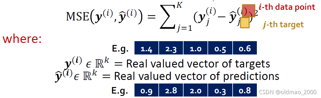
对于N个样本点，总的loss为：
$$Loss=\sum _{i=1}^{N}MSE(y^{(i)},{\hat{y}}^{(i)})$$

Evaluation metrics

Accuracy
ROC AUC
Evaluate regression tasks on graphs:
Root mean square error (RMSE)
$$\sqrt{\sum _{i=1}^N\frac{(y^{(i)}-{\hat{y}}^{(i)}{)}^2}{N}}$$
Mean absolute error (MAE)
$$\frac{{\sum }_{i=1}^N|y^{(i)}-{\hat{y}}^{(i)}|}{N}$$
Evaluate classification tasks on graphs:
多分类直接用准确率，二分类用
§ Accuracy
§ Precision / Recall
§ If the range of prediction is [0,1], we will use 0.5 as threshold
Metric Agnostic to classification threshold
§ ROC AUC

Setting-up GNN Prediction Tasks

主要是数据集的划分，这里的知识点和之前的传统数据集划分有点不一样

固定/随机划分

1. Fixed split: We will split our dataset once
   § Training set: used for optimizing GNN parameters
   § Validation set: develop model/hyperparameters
   § Test set: held out until we report final performance
   A concern: sometimes we cannot guarantee that the test set will really be held out

2. Random split: we will randomly split our dataset into training / validation / test
   § We report average performance over different random seeds

对于传统数据集，由于每个样本之间是相互独立的，但是图数据中节点和节点之间是有边相连的，不是相互独立的，因此划分数据集有两种设置。

Transductive/Inductive setting

The input graph can be observed in all the dataset splits (training, validation and test set).

	Transductive	Inductive
training	we compute embeddings using the entire graph, and train using node 1&2’s labels	we compute embeddings using the graph over node 1&2, and train using node 1&2’s labels
validation	we compute embeddings using the entire graph, and evaluate on node 3&4’s labels	At validation time, we compute embeddings using the graph over node 3&4, and evaluate on node 3&4’s labels
原则	The input graph can be observed in all the dataset splits (training, validation and test set).	We break the edges between splits to get multiple graphs
图例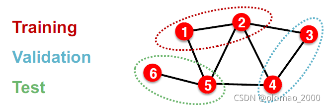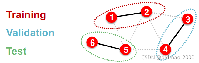
应用	node / edge prediction tasks	node / edge / graph tasks
小结	raining / validation / test sets are on the same graph. The dataset consists of one graph. The entire graph can be observed in all dataset splits,we only split the labels.	training / validation / test sets are on different graphs. The dataset consists of multiple graphs. Each split can only observe the graph(s) within the split. A successful model should generalize to unseen graphs

Transductive/Inductive 划分实例：node classification

Transductive node classification
§ All the splits can observe the entire graph structure, but can only observe the labels of their respective nodes

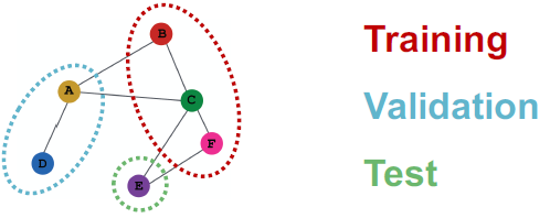
Inductive node classification
§ Suppose we have a dataset of 3 graphs
§ Each split contains an independent graph

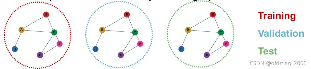
注意，inductive setting 才能做graph classification，Because we have to test on unseen graphs.
Suppose we have a dataset of 5 graphs. Each split will contain independent graph(s).

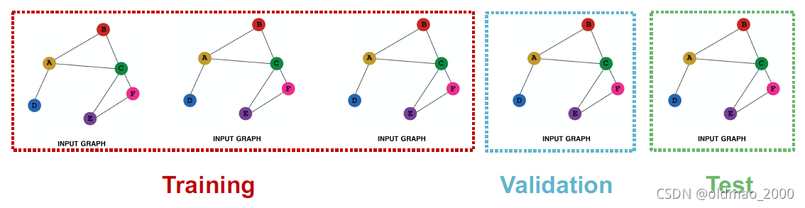
上面看上去一样，但是其实每个数据集给的标签不一样

Transductive/Inductive 划分实例：link prediction

Link prediction is an unsupervised / self-supervised task. We need to create the labels and dataset
splits on our own。就是要自己去掉一些存在的边，然后让模型去预测：

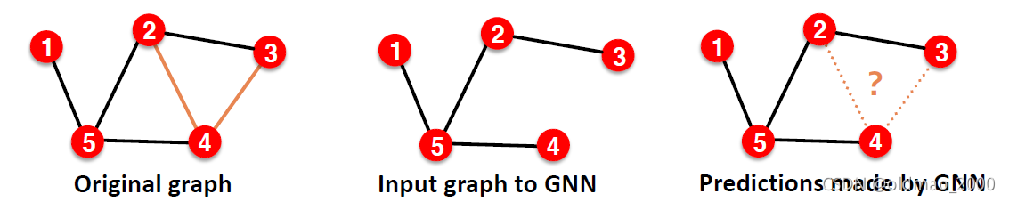
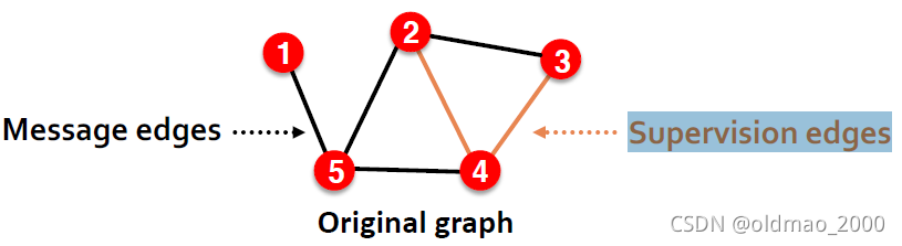
这里把保留的边叫：Message edges，去掉的边叫：Supervision edges

上面这些可以看做是第一步，接下来第二步才是划分数据集，这里分两种：Transductive/Inductive 划分

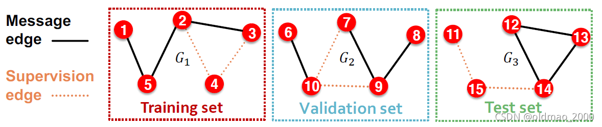
Inductive link prediction split

Suppose we have a dataset of 3 graphs. Each inductive split will contain an independent graph.
In train or val or test set, each graph will have 2 types of edges: message edges + supervision edges

Transductive link prediction split

This is the default setting when people talk about link prediction, the entire graph can be observed in all dataset splits.
Suppose we have a dataset of 1 graph

But since edges are both part of graph structure and the supervision, we need to hold out validation / test edges.
To train the training set, we further need to hold out supervision edges for the training set.

(1) At training time: Use training message edges to predict training supervision edges

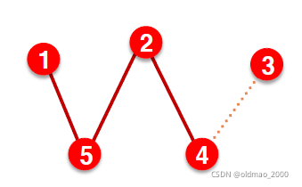
(2) At validation time: Use training message edges & training supervision edges to predict validation edges

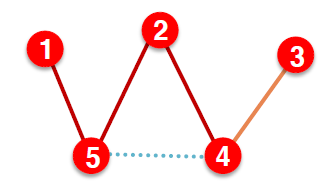
(3) At test time: Use training message edges & training supervision edges & validation edges to predict test edges

After training, supervision edges are known to GNN. Therefore, an ideal model should use supervision edges in message passing at validation time. The same applies to the test time.
是不是看上去很蒙，简单点就是把边分成四类

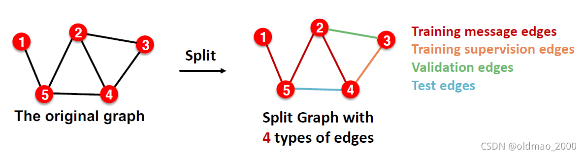
阶段	使用的边	预测的边
训练	Training message edges	Training supervision edges
验证	Training message edges + Training supervision edges	Validation edges
测试	Training message edges + Training supervision edges + Validation edges	Test edges