kaggle房价预测（House Prices: Advanced Regression Techniques）数据分析（一）

这是这个项目的各数据变量的详细解释：https://blog.youkuaiyun.com/Nyte2018/article/details/89977261。
只有对每个变量的意思和分类都了解，才能更好的进行数据分析和处理。
由于本人是这方面的小白，也是第一次参加这种比赛，于是决定选择这个比赛kernels中几篇许多人赞同的数据分析进行学习，这次的kernel是COMPREHENSIVE DATA EXPLORATION WITH PYTHON，在jupyter notebook中运行。

1、准备工作

首先进行各种库的导入：

#invite people for the Kaggle party
import pandas as pd
import matplotlib.pyplot as plt
import seaborn as sns
import numpy as np
from scipy.stats import norm
from sklearn.preprocessing import StandardScaler
from scipy import stats
import warnings
warnings.filterwarnings('ignore')
%matplotlib inline

读取数据集文件：

#bring in the six packs
df_train = pd.read_csv('data/train.csv')

获取数据集中的列名：

#check the decoration
df_train.columns

Index(['Id', 'MSSubClass', 'MSZoning', 'LotFrontage', 'LotArea', 'Street',
       'Alley', 'LotShape', 'LandContour', 'Utilities', 'LotConfig',
       'LandSlope', 'Neighborhood', 'Condition1', 'Condition2', 'BldgType',
       'HouseStyle', 'OverallQual', 'OverallCond', 'YearBuilt', 'YearRemodAdd',
       'RoofStyle', 'RoofMatl', 'Exterior1st', 'Exterior2nd', 'MasVnrType',
       'MasVnrArea', 'ExterQual', 'ExterCond', 'Foundation', 'BsmtQual',
       'BsmtCond', 'BsmtExposure', 'BsmtFinType1', 'BsmtFinSF1',
       'BsmtFinType2', 'BsmtFinSF2', 'BsmtUnfSF', 'TotalBsmtSF', 'Heating',
       'HeatingQC', 'CentralAir', 'Electrical', '1stFlrSF', '2ndFlrSF',
       'LowQualFinSF', 'GrLivArea', 'BsmtFullBath', 'BsmtHalfBath', 'FullBath',
       'HalfBath', 'BedroomAbvGr', 'KitchenAbvGr', 'KitchenQual',
       'TotRmsAbvGrd', 'Functional', 'Fireplaces', 'FireplaceQu', 'GarageType',
       'GarageYrBlt', 'GarageFinish', 'GarageCars', 'GarageArea', 'GarageQual',
       'GarageCond', 'PavedDrive', 'WoodDeckSF', 'OpenPorchSF',
       'EnclosedPorch', '3SsnPorch', 'ScreenPorch', 'PoolArea', 'PoolQC',
       'Fence', 'MiscFeature', 'MiscVal', 'MoSold', 'YrSold', 'SaleType',
       'SaleCondition', 'SalePrice'],
      dtype='object')

2、SalePrice分析

获取saleprice列的详细数据情况：

#descriptive statistics summary
df_train['SalePrice'].describe()

count      1460.000000
mean     180921.195890
std       79442.502883
min       34900.000000
25%      129975.000000
50%      163000.000000
75%      214000.000000
max      755000.000000
Name: SalePrice, dtype: float64

可以看出训练集中一共有1460行数据，平均值为180921.195890等信息。
获取saleprice列的直方图：

#histogram
sns.distplot(df_train['SalePrice']);

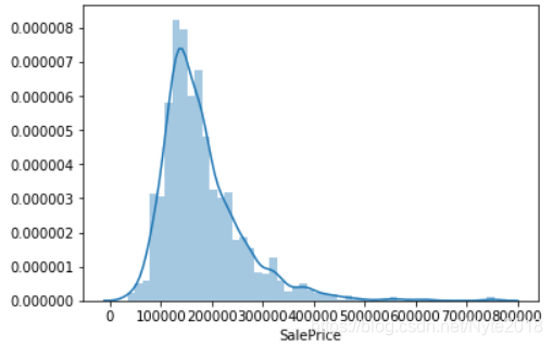
可以看出数据偏离了正态分布，是明显的正偏斜，即偏度大于0。具体的偏度和峰度（反映了峰部的尖度，如果峰度大于三，峰的形状比较尖，比正态分布峰要陡峭）：

#skewness and kurtosis
print("Skewness: %f" % df_train['SalePrice'].skew())
print("Kurtosis: %f" % df_train['SalePrice'].kurt())

Skewness: 1.882876
Kurtosis: 6.536282

3、SalePrice与其它变量的关系

先来看看与数字变量的关系，SalePrice与GrLivArea（地面上居住面积（平方英尺））的关系用散点图表示：

#scatter plot grlivarea/saleprice
var = 'GrLivArea'
data = pd.concat([df_train['SalePrice'], df_train[var]], axis=1)
data.plot.scatter(x=var, y='SalePrice', ylim=(0,800000));

注：pd.concat函数将两列值连接在一起，axis=1表示列合并。

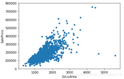
可以看出SalePrice 和 GrLivArea具有线性关系，再看一下和TotalBsmtSF（地下室总面积）的关系：

#scatter plot totalbsmtsf/saleprice
var = 'TotalBsmtSF'
data = pd.concat([df_train['SalePrice'], df_train[var]], axis=1)
data.plot.scatter(x=var, y='SalePrice', ylim=(0,800000));

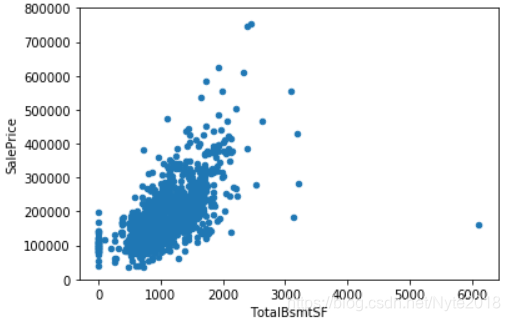
可以看出，SalePrice 和TotalBsmtSF也有线性关系，但是在最左侧，SalePrice的增加和TotalBsmtSF没有关系。
接下来看看与分类特征的关系，此时一般用箱型图。如OverallQual（ 对房子的整体材料和装修进行评级）：

#box plot overallqual/saleprice
var = 'OverallQual'
data