


 本文介绍了CVPR 2018的论文《Deep Back-Projection Networks For Super-Resolution》。核心采用残差学习,介绍了上投影单元、下投影单元、密集上投影单元等方法,阐述了网络架构,包括初始特征提取、反向投影阶段和重建,还提及了细节设置及上采样补充方法。
Deep Back-Projection Networks For Super-Resolution:CVPR 2018
paper:https://arxiv.org/pdf/1803.02735v1.pdf
code:https://github.com/alterzero/DBPN-Pytorch
1. Relative work
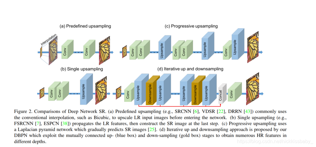
- intro里边提到目前图像SR(超分辨率)的DL模型的四种。分别是
- Predefined upsampling:在进行特征提取前就将图像插值
- Single upsampling:在输出前进行上采样(采用sub-pixel比较好?)
- Progressive upsampling:在特征提取过程中逐步上采样
- Iterative up and downsampling:迭代式的上采样及下采样(本文)
2. Method
核心:残差学习!!!!!
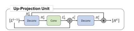
2.1 Up-projection unit
- 公式化
H 0 t = ( L t − 1 ∗ p t ) ↑ s ( 1 ) \quad H_{0}^{t}=\left(L^{t-1} * p_{t}\right) \uparrow_{s} \ \ \ \ (1) H0t=(Lt−1∗pt)↑s (1)
L 0 t = ( H 0 t ∗ g t ) ↓ s ( 2 ) \quad L_{0}^{t}=\left(H_{0}^{t} * g_{t}\right) \downarrow_{s} \ \ \ \ (2) L0t=(H0t∗gt)↓s (2)
e t l = L 0 t − L t − 1 ( 3 ) \quad e_{t}^{l}=L_{0}^{t}-L^{t-1} \ \ \ \ (3) etl=L0t−Lt−1 (3)
H 1 t = ( e t l ∗ q t ) ↑ s ( 4 ) \quad H_{1}^{t}=\left(e_{t}^{l} * q_{t}\right) \uparrow_{s} \ \ \ \ (4) H1t=(etl∗qt)↑s (4)
H t = H 0 t + H 1 t ( 5 ) \quad H^{t}=H_{0}^{t}+H_{1}^{t} \ \ \ \ (5) Ht=H0t+H1t (5)
- L t − 1 L^{t-1} Lt−1 就是上一个Down-projection unit的输出,是当前迭代LR(low-resolution)的原型特征图,将其卷积并上采样得到当前迭代的HR(high-resolution)特征图原型 H 0 t H_{0}^{t} H0t
- 得到HR特征图原型 H 0 t H_{0}^{t} H0t以后怎么得到当前迭代的最终版本的HR特征图呢?答案是学习残差,学习原型 H 0 t H_{0}^{t} H0t到最终版本H^{t}的残差 H 1 t H^{t}_1 H1t
- 怎么学习残差呢?首先将HR原型 H 0 t H_{0}^{t} H0t卷积并下采样得到增强版本的LR特征图 L 0 t L_{0}^{t} L0t。
- 将增强版本的LR特征图 L 0 t L_{0}^{t} L0t与LR原型 L t − 1 L^{t-1} Lt−1 相减得到LR的残差 e t l e_{t}^{l} etl
- 自然地,将LR残差
e
t
l
e_{t}^{l}
etl卷积并上采样便得到了HR残差
H
1
t
H_{1}^{t}
H1t。得到HR残差以后,done
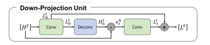
2.2 Down-projection unit
- 公式化
L 0 t = ( H t ∗ g t ′ ) ↓ s ( 6 ) L_{0}^{t}=\left(H^{t} * g_{t}^{\prime}\right) \downarrow_{s} \ \ \ \ (6) L0t=(Ht∗gt′)↓s (6)
H 0 t = ( L 0 t ∗ p t ′ ) ↑ s ( 7 ) H_{0}^{t}=\left(L_{0}^{t} * p_{t}^{\prime}\right) \uparrow_{s} \ \ \ \ (7) H0t=(L0t∗pt′)↑s (7)
e t h = H 0 t − H t ( 8 ) e_{t}^{h}=H_{0}^{t}-H^{t} \ \ \ \ (8) eth=H0t−Ht (8)
L 1 t = ( e t h ∗ g t ′ ) ↓ s ( 9 ) L_{1}^{t}=\left(e_{t}^{h} * g_{t}^{\prime}\right) \downarrow_{s} \ \ \ \ (9) L1t=(eth∗gt′)↓s (9)
L t = L 0 t + L 1 t ( 10 ) L^{t}=L_{0}^{t}+L_{1}^{t} \ \ \ \ (10) Lt=L0t+L1t (10) - down-projection unit的目的是根据上一次迭代的HR特征得到表征力更强的LR特征为下一次的up-projection做准备
- H t H^{t} Ht 就是上一个Up-projection unit的输出,是当前迭代HR(low-resolution)的原型特征图,将其卷积并下采样 L 0 t L_{0}^{t} L0t得到当前迭代的LR(high-resolution)特征图原型
- 得到LR特征图原型 L 0 t L_{0}^{t} L0t以后怎么得到当前迭代的最终版本的LR特征图呢?答案是学习残差,学习原型 L 0 t L_{0}^{t} L0t到最终版本H^{t}的残差 L 1 t L^{t}_1 L1t
- 怎么学习残差呢?首先将LR原型 L 0 t L_{0}^{t} L0t卷积并上采样得到增强版本的HR特征图 H 0 t H_{0}^{t} H0t。
- 将增强版本的HR特征图 H 0 t H_{0}^{t} H0t与HR原型 H t H^{t} Ht相减得到HR的残差 e t h e_{t}^{h} eth
- 自然地,将HR残差 e t h e_{t}^{h} eth卷积并下采样便得到了LR残差 L 1 t L_{1}^{t} L1t。得到LR残差以后,done
- 显然,是up-projection unit的一个逆过程
2.3 Dense Up-projection Unit
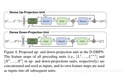
- Dense Up-projection Unit与Up-projection Unit的唯一区别在于输入。Dense Up-projection Unit的输入为浅层的每一个Down-projection unit的输出concat后的特征图。concat以后经过1*1的卷积层降维,再进入一个普通的Up-projection Unit。
- Dense Down-projection Unit同理
2.4 Network Architecture
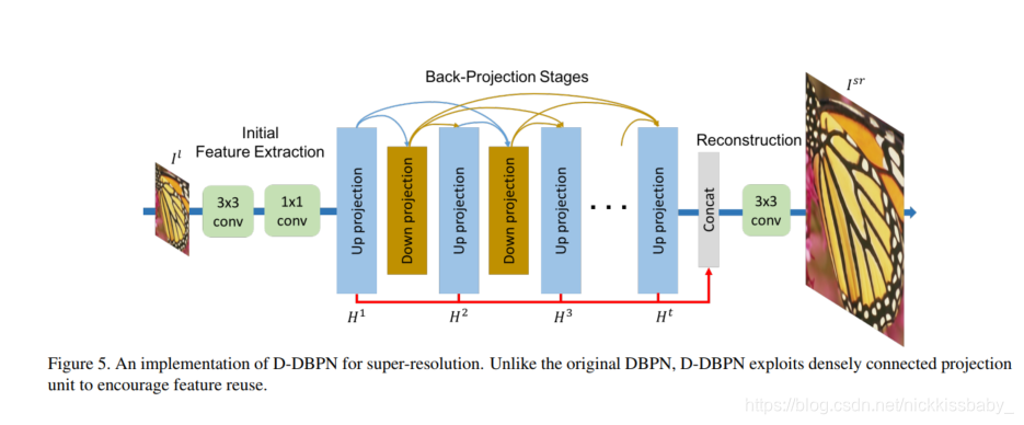
- Initial feature extraction:通过两个3*3的卷积层进行初始化的特征提取
- Back-projection stages:交替式的Up-projection Unit和Down projection Unit积木
- Reconstruction:将所有Up-projection Unit的输出HR特征图concat起来然后进入一个3*3的卷积层,得到最后的HR图片
2.5 Details
- 使用大卷积核
- 2x enlargement:conv 6*6 filters,strides 2 ,padding 2
- 4x enlargement:conv 8*8 filters,strides 4 ,padding 2
- 8x enlargement:conv 12*12 filters,strides 8 ,padding 2
- 抛弃BatchNorm以及Dropout
- Optimizer:adam with momentum 0.9 and weight decay 1e-4
- Loss:MSE
2.6 Supplement
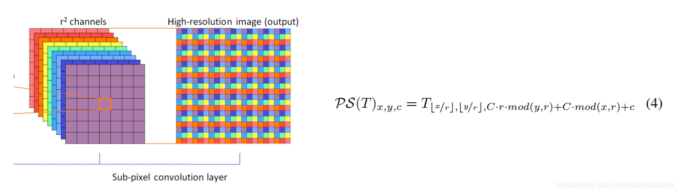
- 本文源码中采用ConvTranspose2d上采样,也可以采用Sub-Pixel(pytorch中为nn.PixelShuffle)进行上采样
- Sub-Pixel由Real-Time Single Image and Video Super-Resolution Using an Efficient Sub-Pixel Convolutional Neural Network 提出


 1026
1026

 被折叠的 条评论
为什么被折叠?
被折叠的 条评论
为什么被折叠?
 到【灌水乐园】发言


