Datawhale组队学习 Task4-建模调参

1. 基础模型

1.1 读取数据

• 知识点1：reduce_mem_usage 函数 对于大量使用数字类型的数据压缩效果很好，主要原理是把int64/float64类型的数值用更小的int(float)32/16/8来搞定，经常会减少50%的内存，甚至是更多

def reduce_mem_usage(df):
    """ iterate through all the columns of a dataframe and modify the data type
        to reduce memory usage.        
    """
    start_mem = df.memory_usage().sum() 
    print('Memory usage of dataframe is {:.2f} MB'.format(start_mem))
    
    for col in df.columns:
        col_type = df[col].dtype
        
        if col_type != object:
            c_min = df[col].min()
            c_max = df[col].max()
            if str(col_type)[:3] == 'int':
                if c_min > np.iinfo(np.int8).min and c_max < np.iinfo(np.int8).max:
                    df[col] = df[col].astype(np.int8)
                elif c_min > np.iinfo(np.int16).min and c_max < np.iinfo(np.int16).max:
                    df[col] = df[col].astype(np.int16)
                elif c_min > np.iinfo(np.int32).min and c_max < np.iinfo(np.int32).max:
                    df[col] = df[col].astype(np.int32)
                elif c_min > np.iinfo(np.int64).min and c_max < np.iinfo(np.int64).max:
                    df[col] = df[col].astype(np.int64)  
            else:
                if c_min > np.finfo(np.float16).min and c_max < np.finfo(np.float16).max:
                    df[col] = df[col].astype(np.float16)
                elif c_min > np.finfo(np.float32).min and c_max < np.finfo(np.float32).max:
                    df[col] = df[col].astype(np.float32)
                else:
                    df[col] = df[col].astype(np.float64)
        else:
            df[col] = df[col].astype('category')

    end_mem = df.memory_usage().sum() 
    print('Memory usage after optimization is: {:.2f} MB'.format(end_mem))
    print('Decreased by {:.1f}%'.format(100 * (start_mem - end_mem) / start_mem))
    return df

sample_feature = reduce_mem_usage(pd.read_csv('data_for_tree.csv'))
continuous_feature_names = [x for x in sample_feature.columns if x not in ['price','brand','model','brand']]

1.2 线性回归

1.2.1 初试

• 知识点2：sorted(d.items(), key=lambda x: x[1]) d.items()为待排序对象，key=key=lambda x: x[1] 为对前面的对象中的第二维数据（value）进行排序
• 知识点3：np.random.randint(low, high=None, size=None, dtype=‘l’) 返回随机整数，范围[low, high)

# (1)数据集载入
sample_feature = sample_feature.dropna().replace('-', 0).reset_index(drop=True)
sample_feature['notRepairedDamage'] = sample_feature['notRepairedDamage'].astype(np.float32)
train = sample_feature[continuous_feature_names+['price']]
train_x = train[continuous_feature_names]
train_y = train['price']

# (2)建模
model = LinearRegression(normalize=True)
model = model.fit(train_x, train_y)
# (3)查看intercept-截距和coef-权重
print('intercept'+str(model.intercept_))
print(sorted(dict(zip(continuous_feature_names, model.coef_)).items(), key=lambda x:x[1], reverse=True))
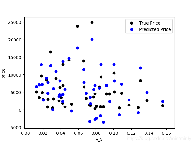
# 通过绘制特征v_9的值与标签的散点图，可以发现预测值（蓝）和真实值（黑）分布差异较大，且预测值出现<0情况，说明模型存在一些问题
subsample_index = np.random.randint(low=0, high=len(train_y), size=50)
plt.scatter(train_x['v_9'][subsample_index],train_y[subsample_index],color='black')
plt.scatter(train_x['v_9'][subsample_index],model.predict(train_x.loc[subsample_index]),color='blue')
plt.xlabel('v_9')
plt.ylabel('price')
plt.legend(['True Price','Predicted Price'],loc='upper right')
print('The predicted price is obvious different from true price')
plt.show()

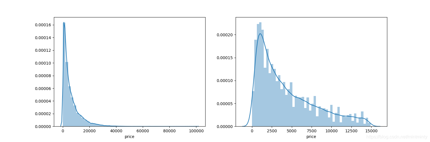
# (4)观察长尾分布
print('It is clear to see the price shows a typical exponential distribution')
plt.figure(figsize=(15,5))
plt.subplot(1,2,1)  # plt.subplot(nrows, ncols, index, **kwargs)
sns.distplot(train_y)
plt.subplot(1,2,2)
sns.distplot(train_y[train_y < np.quantile(train_y, 0.9)])

1.2.2 改进

• 从上图可看出，预测值（蓝）和真实值（黑）分布差异较大，且预测值出现<0情况，说明模型存在一些问题。
• 原因是很多模型都假设数据误差项符合正态分布，而标签数据（price）呈现长尾分布违背该假设。（详情见参考链接1或task2笔记）

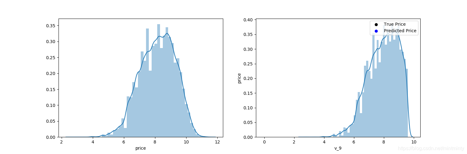
# (1)对标签进行log(x+1)变换，使标签贴近于正态分布
train_y_ln = np.log(train_y + 1)
# (2)观察变换后的数据分布
print('The transformed price seems like normal distribution')
plt.figure(figsize=(15,5))
plt.subplot(1,2,1)
sns.distplot(train_y_ln)
plt.subplot(1,2,2)
sns.distplot(train_y_ln[train_y_ln < np.quantile(train_y_ln, 0.9)])
# (3)拟合模型
model = model.fit(train_x,train_y_ln)
print('intercept'+str(model.intercept_))
print(sorted(dict(zip(continuous_feature_names, model.coef_)).items(), key=lambda x:x[1], reverse=True))
# (4)绘制真实值、预测值
plt.scatter(train_x['v_9'][subsample_index], train_y[subsample_index],color='black')
plt.scatter(train_x['v_9'][subsample_index], np.exp(model.predict(train_x.loc[subsample_index])),color='blue')  # 预测值要记得变换回去
plt.xlabel('v_9')
plt.ylabel('price')
plt.legend(['True Price','Predicted Price'],loc='upper right')
print('The predicted price seems normal after np.log transforming')
plt.show()

1.3 五折交叉验证

• 知识点5：cross_val_score()参数

参数	意义
estimator	估计方法对象(分类器)
x	数据特征features
y	数据标签labels
scoring	调用方法
cv	几折交叉验证
n_jobs	同时工作cpu个数(-1表示全部）
verbose	详细程度

def log_transfer(func):
    def wrapper(y, yhat):
        result = func(np.log(y), np.nan_to_num(np.log(yhat)))
        return result
    return wrapper

"""
# 用未去长尾化的数据进行五折交叉验证(Error 1.36)
scores = cross_val_score(model, x=train_x, y=train_y, verbose=1, cv=5, scoring=make_scorer(log_transfer(mean_absolute_error)))
print('AVG:', np.mean(scores))
"""
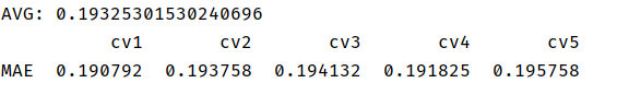
# 用去长尾化的数据进行无折交叉验证(Error 0.19)
scores = cross_val_score(model, X=train_x, y=train_y_ln, verbose=1, cv = 5, scoring=make_scorer(mean_absolute_error))
print('AVG:', np.mean(scores))
scores = pd.DataFrame(scores.reshape(1,-1))
scores.columns = ['cv'+str(x) for x in range(1,6)]
scores.index = ['MAE']
print(scores)

1.4 模拟真实业务情况

五折交叉验证在某些与时间相关的数据集上反映了不真实的情况，通过2018年的二手车价格预测2017年的二手车价格，显然是不合理的，因此我们采用时间顺序对数据集进行分割，选用靠前时间的4/5样本作为训练集，靠后时间的1/5作为验证集

• 知识点6：np.linspace()

参数	意义
start	队列的开始值
stop	队列的结束值
num	生成的样本数，默认50
endpoint	默认True，包含右区间
retstep	默认False，返回等差数列；否则返回array([samples, step])

• 知识点7：learning_curve()

参数	意义
estimator	所使用的分类器
x	数据特征features
y	数据标签labels
train_size	训练样本的绝对/相对数量
cv	几折交叉验证
ylim	定义绘制的最小和最大y值

• 知识点8：plt.fill_between(x, y1, y2, facecolor=‘green’, alpha=0.3)，即y1和y2之间颜色填充

# (1)模拟真实业务情况
sample_feature = sample_feature.reset_index(drop=True)  # reset_index(drop=True)删除原索引
split_point = len(sample_feature)//5*4
train = sample_feature.loc[:split_point].dropna()
val = sample_feature.loc[:split_point].dropna()
train_x = train[continuous_feature_names]
train_y_ln = np.log(train['price'] + 1)
val_x = val[continuous_feature_names]
val_y_ln = np.log(val['price'] + 1)

model = model.fit(train_x,train_y_ln)
mean_absolute_error(val_y_ln, model.predict(val_x))


# (2)学习率曲线与验证曲线
def plot_learning_curve(estimator, title, x, y, ylim=None, cv=None,n_jobs=1,train_size=np.linspace(.1, 1.0, 5 )):
    plt.figure()
    plt.title(title)
    if ylim is not None:
        plt.ylim(*ylim)
    plt.xlabel('Training example')
    plt.ylabel('score')
    train_sizes, train_scores, test_scores = learning_curve(estimator, x, y, cv=cv, n_jobs=n_jobs,\
                                                            train_sizes=train_size,\
                                                            scoring=make_scorer(mean_absolute_error))
    train_scores_mean = np.mean(train_scores, axis=1)
    train_scores_std = np.std(train_scores, axis=1)
    test_scores_mean = np.mean(test_scores, axis=1)
    test_scores_std = np.std(test_scores, axis=1)
    plt.grid()
    plt.plot(train_sizes,train_scores_mean,'o-',color='r',label='Training score')
    plt.plot(train_sizes, test_scores_mean, 'o-', color="g",label="Cross-validation score")
    plt.fill_between(train_sizes,train_scores_mean-train_scores_std,train_scores_mean+train_scores_std,alpha=0.1,color='r')
    plt.fill_between(train_sizes,test_scores_mean-test_scores_std,test_scores_mean+test_scores_std,alpha=0.1,color='g')
    plt.legend(loc='best')
    return plt


plot_learning_curve(LinearRegression(), 'Linear_model', train_x[:1000], train_y_ln[:1000], ylim=(0.0, 0.5), cv=5, n_jobs=1)

2. 对比模型

2.1 线性模型+嵌入式特征

• 加上所有参数（不包括${\theta }_0$）的绝对值之和，即$l_1$范数，为Lasso回归
• 加上所有参数（不包括${\theta }_0$）的平方和，即$l_2$范数，为岭回归

注：在这部分训练时程序报错，后来经过查询发现是“notRepairedDamage”属性下存在空值，于是对空值进行了删除处理。（大概是我之前保存数据出了问题…好坑，找了好长时间问题QAQ）

# 2.1 线性模型+嵌入式特征选择
train = sample_feature[continuous_feature_names + ['price']]
train['notRepairedDamage'].replace('-', np.nan, inplace=True)
train = train[continuous_feature_names + ['price']].dropna(axis=0, how='any')

train_x = train[continuous_feature_names]
train_y = train['price']
train_y_ln = np.log(train_y + 1)

models = [LinearRegression(), Ridge(), Lasso()]
result = dict()
for model in models:
    model_name = str(model).split('(')[0]
    scores = cross_val_score(model, X=train_x, y=train_y_ln, verbose=0, cv = 5,scoring=make_scorer(mean_absolute_error))
    result[model_name] = scores
    print(model_name + ' is finished')
result = pd.DataFrame(result)
result.index = ['cv' + str(x) for x in range(1, 6)]
print(result)

model = LinearRegression().fit(train_x, train_y_ln)
print('intercept'+str(model.intercept_))
plt.figure(figsize=(10,15))
sns.barplot(abs(model.coef_),continuous_feature_names)
plt.savefig('lr权重.png',dpi=600)

model = Ridge().fit(train_x, train_y_ln)
print('intercept:'+ str(model.intercept_))
plt.figure(figsize=(10,15))
sns.barplot(abs(model.coef_),continuous_feature_names)
plt.savefig('ridge权重.png',dpi=600)

model = Lasso().fit(train_x, train_y_ln)
print('intercept:'+ str(model.intercept_))
sns.barplot(abs(model.coef_), continuous_feature_names)
plt.figure(figsize=(10,15))
sns.barplot(abs(model.coef_),continuous_feature_names)
plt.savefig('lasso权重.png',dpi=600)

LinearRegression

L1正则化：Lasso

• 有助于生成一个稀疏权值矩阵，进而用于特征选择，L1范数被称为“稀疏规则算子”
• 由下图可知，power与userd_time特征非常重要
  

L2正则化：Ridge

• 主要解决过拟合问题，使得权重趋近于0，但是不会为0
• 模型的参数比较小，说明模型简单，泛化能力强。解释：可以设想一下对于一个线性回归方程，若参数很大，那么只要数据偏移一点点，就会对结果造成很大的影响；但如果参数足够小，数据偏移得多一点也不会对结果造成什么影响，专业一点的说法——抗扰动能力强。
• 参数比较小，说明某些多项式分支的作用很小，降低了模型的复杂程度

2.2 非线性模型

models = [LinearRegression(),
          DecisionTreeRegressor(),
          RandomForestRegressor(),
          GradientBoostingRegressor(),
          MLPRegressor(solver='lbfgs', max_iter=100), 
          XGBRegressor(n_estimators = 100, objective='reg:squarederror'), 
          LGBMRegressor(n_estimators = 100)]
result = dict()
for model in models:
    model_name = str(model).split('(')[0]
    scores = cross_val_score(model, X=train_X, y=train_y_ln, verbose=0, cv = 5, scoring=make_scorer(mean_absolute_error))
    result[model_name] = scores
    print(model_name + ' is finished')
result = pd.DataFrame(result)
result.index = ['cv' + str(x) for x in range(1, 6)]
print(result)

3. 模型调参

3.1 贪心算法

objective = ['regression','regression_l1', 'mape', 'huber', 'fair' ]
num_leaves = [3,5,10,15,20,40, 55]
max_depth = [3,5,10,15,20,40, 55]
bagging_fraction = []
feature_fraction = []
drop_rate = []

best_obj = dict()
for obj in objective:
    model = LGBMRegressor(objective=obj)
    score = np.mean(cross_val_score(model, X=train_x, y=train_y_ln, verbose=0, cv = 5, scoring=make_scorer(mean_absolute_error)))
    best_obj[obj]=score

best_leaves = dict()
for leaves in num_leaves:
    model = LGBMRegressor(objective=min(best_obj.items(), key=lambda x: x[1])[0], num_leaves=leaves)
    score = np.mean(cross_val_score(model, X=train_x, y=train_y_ln, verbose=0, cv=5, scoring=make_scorer(mean_absolute_error)))
    best_leaves[leaves] = score

best_depth = dict()
for depth in max_depth:
    model = LGBMRegressor(objective=min(best_obj.items(), key=lambda x:x[1])[0],\
                          num_leaves=min(best_leaves.items(), key=lambda x:x[1])[0],\
                          max_depth=depth)
    score = np.mean(cross_val_score(model, X=train_x, y=train_y_ln, verbose=0, cv = 5, scoring=make_scorer(mean_absolute_error)))
    best_depth[depth] = score

sns.lineplot(x=['0_initial','1_turning_obj','2_turning_leaves','3_turning_depth'], y=[0.143 ,min(best_obj.values()), min(best_leaves.values()), min(best_depth.values())])
 

3.2 网格调参

• 网格调参：在指定的范围内可以自动调参，只需将参数输入即可得到最优化的结果和参数
• GridSearchCV(estimator, param_grid, scoring=None, fit_params=None, n_jobs=1, iid=True, refit=True, cv=None, verbose=0, pre_dispatch=‘2*n_jobs’, error_score=‘raise’, return_train_score=True)

参数	意义
estimator	分类器类别
param_grid	需要最优化的参数的取值，值为字典或列表
scoring	准确度评价标准，默认为None，根据所选模型不同，评价准则不同，如可以选择scoring='accuracy’或者’roc_auc’等
cv	交叉验证折数
refit	默认为True，即在搜索参数结束后，用最佳参数结果再次fit一遍全部数据集
iid	默认为True，误差估计为所有样本的和，而非各个fold的平均

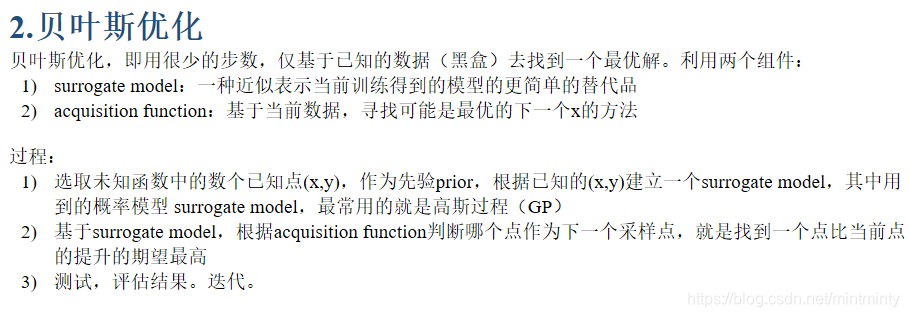
3.3 贝叶斯调参

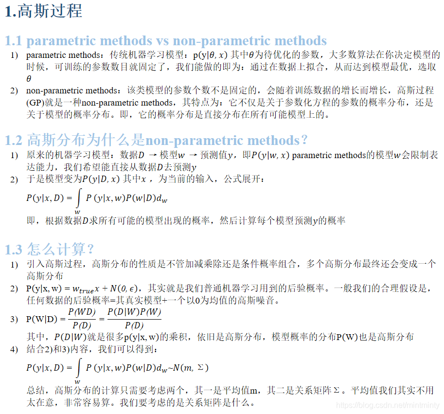
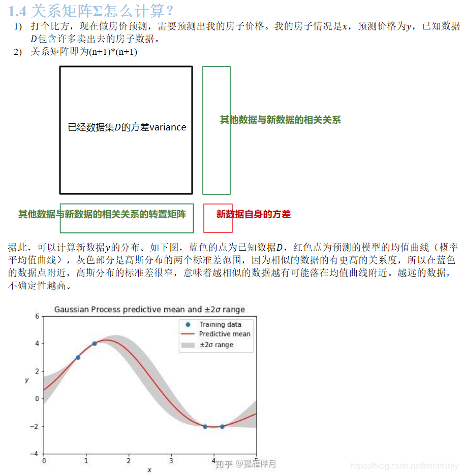
• 是基于数据使用贝叶斯定理估计目标函数的后验分布，然后再根据分布选择下一个采样的超参数组合。
• 这个贝叶斯优化，说实话我感觉原理上并没有完全看懂，下文是基于参考连接【7】【8】的总结，个人感觉原博写得很好，但是自己的理解还没有完全打通的感觉…QAQ
  
  
  

def rf_cv(num_leaves, max_depth, subsample, min_child_samples):
    val = cross_val_score(
        LGBMRegressor(objective = 'regression_l1',
            num_leaves=int(num_leaves),
            max_depth=int(max_depth),
            subsample = subsample,
            min_child_samples = int(min_child_samples)
        ),
        X=train_X, y=train_y_ln, verbose=0, cv = 5, scoring=make_scorer(mean_absolute_error)
    ).mean()
    return 1 - val

rf_bo = BayesianOptimization(
    rf_cv,
    {
    'num_leaves': (2, 100),
    'max_depth': (2, 100),
    'subsample': (0.1, 1),
    'min_child_samples' : (2, 100)
    }
)

print(rf_bo.maximize())

【参考链接】

【1】回归分析的五个基本假设
【2】learning_curve()使用文档
【3】plt.fill_between()函数
【4】正则化的线性回归 —— 岭回归与Lasso回归
【5】L1,L2正则化的原理与区别
【6】Python-sklearn包中自动调参方法-网格搜索GridSearchCV
【7】贝叶斯优化（Bayesian Optimization）（一）：高斯过程（GP）
【8】贝叶斯优化（Bayesian Optimization）（二）：贝叶斯优化