


实验一 线性模型
1.实验目的
1、掌握线性模型(岭回归)在回归任务中的相应理论与应用。
2、掌握线性模型(LDA模型)在分类任务中的相应理论与应用。
2.回归任务
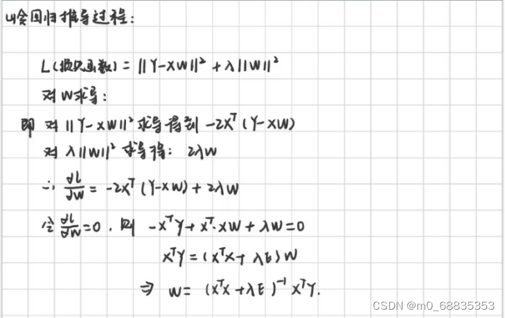
01 岭回归模型对应数学公式推导过程
02 编写程序实现岭回归模型,并对代码进行注释说明
clc;clear;close all;
load('data.mat')
n=size(data,2);
x=data(:,1:n-1); %自变量
y=data(:,n); %因变量
xm=mean(x); %x的平均值
xs=std(x); %x的方差
ym=mean(y); %y的平均值
%原自变量的多元线性回归
x_o=zscore(x);
k1=[1:0.1:10];
for k=1:length(k1)
%用标准化后的进行多元线性回归
lamda=k1(k);
xishu=(x_o'*x_o+lamda*eye(size(x_o,2)))^(-1)*x_o'*(y-ym);
%还原为原自变量的系数
xishu1=[ym-sum(xishu.*xm'./xs');xishu./xs'];
y_n1=xishu1(1)+x*xishu1(2:end);
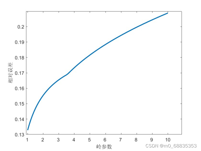
wucha(k)=sum(abs(y_n1-y)./y)/length(y);
end
plot(wucha,'LineWidth',2)
ylabel('相对误差')
xlabel('岭参数')
set(gca,'XTick',1:10:100)
set(gca,'XtickLabel',1:1:10)
clc;clear;close all;
load('data.mat')
n=size(data,2);
x=data(:,1:n-1);
y=data(:,n);
k = 1:0.1:10;
B = ridge(y,x,k,0);
%B = ridge(y,X,k,scaled);
%k为岭参数,scaled为标准化的范围
figure(1)
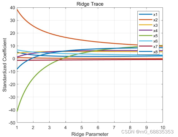
plot(k,B,'LineWidth',2)
legend('x1','x2','x3','x4','x5','x6','x7','x8')
%ylim([-100 100])
grid on
xlabel('Ridge Parameter')
ylabel('Standardized Coefficient')
title('Ridge Trace')
for k1 = 1:length(k)
A=B(:,k1);
yn= A(1)+x*A(2:end);
wucha(k1)=sum(abs(y-yn)./y)/length(y);
end
figure(2)
subplot(2,1,1)
plot(1:length(k),wucha,'LineWidth',2)
ylabel('相对误差')
xlabel('岭参数')
set(gca,'XTick',1:10:100)
set(gca,'XtickLabel',1:1:10)
subplot(2,1,2)
index=find(wucha==min(wucha));
xishu = ridge(y,x,k(index),0);
y_p= A(1)+x*A(2:end);
color1=[184 184 246]/255;
color2=[255 193 151]/255;
titlestr=['岭参数取值为:',num2str(k(index)),' 误差为:',num2str(min(wucha))];
plot(y(3000:end),'Color',color1,'LineWidth',1)
hold on
plot(y_p(3000:end),'*','Color',color2)
hold on
legend('真实数据','多元线性回归拟合数据')
title(titlestr)
3.分类任务
01 LDA模型对应数学公式推导过程

02 写程序实现岭回归模型,并对代码进行注释与说明
function [W] = FisherLDA(w1,w2)

mu1=mean(w1);
mu2=mean(w2);
mu=mean([w1;w2]);

n1=size(w1,1);
n2=size(w2,1);

S1=0;
for i=1:n1
S1=S1+(w1(i,:)-mu1)'*(w1(i,:)-mu1);
end

S2=0;
for i=1:n2
S2=S2+(w2(i,:)-mu2)'*(w2(i,:)-mu2);
end
Sw=S1+S2;

Sb=(n1*(mu-mu1)'*(mu-mu1)+n2*(mu-mu2)'*(mu-mu2))/(n1+n2);

[V,D]=eig(inv(Sw )*Sb);
[~,b]=max(max(D));
W=V(:,b);
end

clc;clear;close all;
%LDA分类主程序
clear all, close all,
cls1_data=[2.532 6.798; 2.952 6.531;3.268 5.471; 3.572 5.658];
cls2_data=[2.121 4.232; 2.265 6.227; 2.583 3.468;3.078 3.522];

plot(cls1_data(:,1),cls1_data(:,2),'*r');
hold on;
plot(cls2_data(:,1),cls2_data(:,2),'ob');
w=FisherLDA(cls1_data,cls2_data);

new1=cls1_data*w;
new2=cls2_data*w;
k=w(2)/w(1);
plot([0,6],[0,6*k],'-k');

axis([2 6 0 11]);

for i=1:4
tmp=cls1_data(i,:);
newx=(tmp(1)+k*tmp(2))/sqrt(k^2+1);

newy=k*newx;
plot(newx,newy,'*r');
end
for i=1:4
tmp=cls2_data(i,:);
newx=(tmp(1)+k*tmp(2))/sqrt(k^2+1);

newy=k*newx;
plot(newx,newy,'ob');
end
hold off
legend('Class 1','Class 2','Location','SE')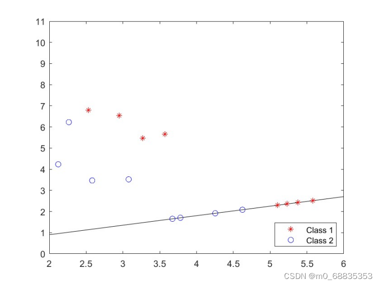


 被折叠的 条评论
为什么被折叠?
被折叠的 条评论
为什么被折叠?
 到【灌水乐园】发言


