


目录
一、自我训练
1、分类的例子
# 自我训练——分类

import numpy as np
from sklearn.ensemble import RandomForestClassifier
from sklearn.semi_supervised import SelfTrainingClassifier
from sklearn.model_selection import train_test_split
from sklearn.datasets import make_classification

# 生成示例数据:部分标签缺失
X, y = make_classification(n_samples=1000, n_features=20, n_informative=15, random_state=42)


# 划分训练集与测试集(测试集全部有标签)
X_train, X_test, y_train, y_test = train_test_split(X, y, test_size=0.2, random_state=42)

# 随机将训练集70%的标签设置为-1表示无标签
rng = np.random.RandomState(42)
random_unlabeled_points = rng.rand(len(y_train)) < 0.7
y_train[random_unlabeled_points] = -1


# 初始化基本分类器(例如随机森林)
base_clf = RandomForestClassifier(n_estimators=100, random_state=42)

# 用自我训练方法封装基本分类器
self_training_clf = SelfTrainingClassifier(base_clf, threshold=0.8, criterion='threshold')

# 训练模型
self_training_clf.fit(X_train, y_train)

# 评估性能
print("Test accuracy:", self_training_clf.score(X_test, y_test))
Test accuracy: 0.835
2、回归的例子
# 自我训练——回归


import numpy as np
from sklearn.ensemble import RandomForestRegressor
from sklearn.datasets import make_regression
from sklearn.model_selection import train_test_split
from sklearn.metrics import mean_squared_error

# 生成回归数据
X, y = make_regression(n_samples=1000, n_features=20, noise=10, random_state=42)

# 划分训练集和测试集(测试集保留完整标签)
X_train, X_test, y_train_full, y_test = train_test_split(X, y, test_size=0.2, random_state=42)

# 模拟训练集中70%的样本无标签,设为NaN表示缺失标签
rng = np.random.RandomState(42)
mask = rng.rand(len(y_train_full)) < 0.9
y_train = y_train_full.copy()
y_train[mask] = np.nan

# 定义函数:利用随机森林各决策树的预测计算均值和标准差
def predict_with_std(rf, X):
    # 获取每棵树的预测结果
    preds = np.array([est.predict(X) for est in rf.estimators_])
    mean_preds = preds.mean(axis=0)
    std_preds = preds.std(axis=0)
    return mean_preds, std_preds

# 初始化基本回归器
base_regressor = RandomForestRegressor(n_estimators=100, random_state=42)

# 自我训练(伪标签)参数设置
max_iterations = 10
confidence_threshold = 120  # 阈值,标准差低于此值认为预测置信度高

# 用布尔数组记录哪些样本已标注(包括真实标签和伪标签)
labeled_mask = ~np.isnan(y_train)

for iteration in range(max_iterations):
    # 用当前标注样本训练回归器
    base_regressor.fit(X_train[labeled_mask], y_train[labeled_mask])

    # 找出无标签样本的索引
    unlabeled_indices = np.where(~labeled_mask)[0]
    if len(unlabeled_indices) == 0:
        break

    X_unlabeled = X_train[unlabeled_indices]

    # 利用模型对无标签数据进行预测,同时获得预测标准差
    pseudo_preds, std_preds = predict_with_std(base_regressor, X_unlabeled)

    # 选取预测标准差低于阈值的样本,认为预测可信
    #print(std_preds)
    confident_mask = std_preds < confidence_threshold
    if not confident_mask.any():
        print(f"Iteration {iteration}: No confident predictions, stopping.")
        break

    # 更新这些样本的标签为伪标签
    confident_indices = unlabeled_indices[confident_mask]
    y_train[confident_indices] = pseudo_preds[confident_mask]
    labeled_mask = ~np.isnan(y_train)  # 更新标注状态

    print(f"Iteration {iteration}: Added {len(confident_indices)} pseudo-labeled samples.")

# 最终模型在测试集上评估
y_pred_test = base_regressor.predict(X_test)


mse = mean_squared_error(y_test, y_pred_test)
print("Test MSE:", mse)
Iteration 0: Added 24 pseudo-labeled samples.
Iteration 1: Added 99 pseudo-labeled samples.
Iteration 2: Added 240 pseudo-labeled samples.
Iteration 3: Added 211 pseudo-labeled samples.
Iteration 4: Added 111 pseudo-labeled samples.
Iteration 5: Added 17 pseudo-labeled samples.
Iteration 6: Added 1 pseudo-labeled samples.
Iteration 7: Added 1 pseudo-labeled samples.
Iteration 8: No confident predictions, stopping.
Test MSE: 19191.928223350456
二、协同训练
# 协同训练

import numpy as np
from sklearn.naive_bayes import GaussianNB
from sklearn.metrics import accuracy_score
from sklearn.model_selection import train_test_split
from sklearn.datasets import make_classification

# 构造示例数据(假设特征可以分成两组)
def split_features(X):
    # 假设前一半为视角1,后一半为视角2
    d = X.shape[1] // 2
    return X[:, :d], X[:, d:]

X, y = make_classification(n_samples=500, n_features=20, n_informative=10, random_state=42)
X_view1, X_view2 = split_features(X)

# 随机设置部分样本无标签 (-1 表示未知标签)
rng = np.random.RandomState(42)
y_co = y.copy()
unlabeled_mask = rng.rand(len(y)) < 0.7
y_co[unlabeled_mask] = -1

# 划分训练(带标签)和无标签数据
labeled_idx = np.where(y_co != -1)[0]
unlabeled_idx = np.where(y_co == -1)[0]

X1_labeled, X2_labeled = X_view1[labeled_idx], X_view2[labeled_idx]
y_labeled = y[labeled_idx]

X1_unlabeled, X2_unlabeled = X_view1[unlabeled_idx], X_view2[unlabeled_idx]

# 初始化两个视角的分类器
clf1 = GaussianNB()
clf2 = GaussianNB()

# 初始训练:仅使用带标签数据
clf1.fit(X1_labeled, y_labeled)
clf2.fit(X2_labeled, y_labeled)

# 协同训练迭代次数
n_iter = 5
for it in range(n_iter):
    # 分别在无标签数据上进行预测
    pseudo_labels1 = clf1.predict(X1_unlabeled)
    pseudo_labels2 = clf2.predict(X2_unlabeled)

    # 找出两个分类器预测一致的样本作为高置信样本
    agreed = pseudo_labels1 == pseudo_labels2
    if np.sum(agreed) == 0:
        break
    X1_new = X1_unlabeled[agreed]
    X2_new = X2_unlabeled[agreed]
    y_new = pseudo_labels1[agreed]

    # 将这些高置信样本加入带标签数据中
    X1_labeled = np.vstack([X1_labeled, X1_new])
    X2_labeled = np.vstack([X2_labeled, X2_new])
    y_labeled = np.concatenate([y_labeled, y_new])

    # 移除已添加的无标签样本
    keep_mask = ~agreed
    X1_unlabeled = X1_unlabeled[keep_mask]
    X2_unlabeled = X2_unlabeled[keep_mask]

    # 重新训练两个分类器
    clf1.fit(X1_labeled, y_labeled)
    clf2.fit(X2_labeled, y_labeled)

    print(f"Iteration {it+1}: Added {len(y_new)} pseudo-labeled samples.")

# 最终模型可以对新数据的两个视角分别预测,然后投票决定最终类别
Iteration 1: Added 209 pseudo-labeled samples.
Iteration 2: Added 38 pseudo-labeled samples.
Iteration 3: Added 7 pseudo-labeled samples.
Iteration 4: Added 1 pseudo-labeled samples.
三、生成式模型GMM
# 生成式模型GMM

import numpy as np
from sklearn.datasets import make_classification
from sklearn.metrics import accuracy_score
from scipy.stats import multivariate_normal

# 1. 生成数据
# 生成一个二分类问题的数据集
X, y_true = make_classification(n_samples=1000, n_features=10, n_informative=5,
                                n_clusters_per_class=1, random_state=42)

# 模拟半监督场景:80%的标签设为 -1 表示缺失
rng = np.random.RandomState(42)
y = y_true.copy()
unlabeled_mask = rng.rand(len(y)) < 0.8
y[unlabeled_mask] = -1

# 获取带标签数据的索引
labeled_idx = np.where(y != -1)[0]
print("有标签数据数:", len(labeled_idx))

# 2. 初始化参数
# 假设类别数与真实类别数一致(K=2)
K = len(np.unique(y_true))
n_samples, n_features = X.shape

# 初始化混合系数、均值和协方差矩阵
pi = np.zeros(K)
mu = np.zeros((K, n_features))
Sigma = np.zeros((K, n_features, n_features))
for k in range(K):
    # 利用带标签数据初始化参数
    X_k = X[y == k]
    if len(X_k) > 0:
        pi[k] = len(X_k) / n_samples
        mu[k] = np.mean(X_k, axis=0)
        # 保证协方差矩阵非奇异
        Sigma[k] = np.cov(X_k.T) + np.eye(n_features)*1e-6
    else:
        # 如果某个类别没有带标签样本,则随机初始化
        pi[k] = 1.0 / K
        mu[k] = np.random.randn(n_features)
        Sigma[k] = np.eye(n_features)

# 3. EM 算法迭代(半监督版)
max_iter = 50
tol = 1e-5

# 用于存储每个样本对每个高斯成分的责任
gamma = np.zeros((n_samples, K))

for iteration in range(max_iter):
    # E 步骤:计算责任
    for i in range(n_samples):
        if y[i] != -1:
            # 对于有标签数据,强制其责任只落在真实类别上
            gamma[i] = np.zeros(K)
            gamma[i, y[i]] = 1.0
        else:
            # 对于无标签数据,根据当前模型计算后验概率
            probs = np.array([pi[k] * multivariate_normal.pdf(X[i], mean=mu[k], cov=Sigma[k])
                              for k in range(K)])
            # 防止数值下溢
            if probs.sum() == 0:
                probs = np.ones(K)
            gamma[i] = probs / probs.sum()

    # M 步骤:根据责任更新参数
    pi_new = gamma.sum(axis=0) / n_samples
    mu_new = np.zeros_like(mu)
    Sigma_new = np.zeros_like(Sigma)

    for k in range(K):
        N_k = gamma[:, k].sum()  # 某一成分的有效样本数
        if N_k > 0:
            mu_new[k] = np.sum(gamma[:, k][:, None] * X, axis=0) / N_k
            diff = X - mu_new[k]
            Sigma_new[k] = np.dot((gamma[:, k][:, None] * diff).T, diff) / N_k
            # 加入正则项避免协方差矩阵奇异
            Sigma_new[k] += np.eye(n_features) * 1e-6
        else:
            mu_new[k] = mu[k]
            Sigma_new[k] = Sigma[k]

    # 判断是否收敛,这里用均值变化作为衡量标准
    if np.linalg.norm(mu_new - mu) < tol:
        print("收敛于迭代次数:", iteration)
        break

    # 更新参数
    pi = pi_new
    mu = mu_new
    Sigma = Sigma_new

# 4. 预测与评估
# 根据最终的责任分布,将每个样本分配到后验概率最大的成分
y_pred = np.argmax(gamma, axis=1)

# 仅在有标签数据上评估分类准确率
accuracy = accuracy_score(y_true[labeled_idx], y_pred[labeled_idx])
print("半监督生成模型在有标签数据上的准确率:", accuracy)
有标签数据数: 199
收敛于迭代次数: 6
半监督生成模型在有标签数据上的准确率: 1.0
四、基于图的半监督算法-标签传播
# 基于图的半监督算法-标签传播
import numpy as np
from sklearn.datasets import load_iris
from sklearn.semi_supervised import LabelSpreading
from sklearn.metrics import accuracy_score
import matplotlib.pyplot as plt
# 1. 加载数据
iris = load_iris()
X = iris.data
y_true = iris.target # 保存真实标签
y = np.copy(y_true)
print("总样本数:",len(y))
# 2. 模拟半监督场景:随机将50%的标签置为未标注(-1)
rng = np.random.RandomState(42)
mask = rng.rand(len(y)) < 0.5 # 50%概率
y[mask] = -1
print("有标签样本数量:", np.sum(y != -1))
# 3. 构建并训练 LabelSpreading 模型
# 使用基于k近邻的核函数,构造样本间的图
label_spread = LabelSpreading(kernel='knn', n_neighbors=7, alpha=0.2)
label_spread.fit(X, y)
# 4. 获取传播后的标签
y_pred = label_spread.transduction_
# 5. 评估效果:仅在原有标签(置为 -1)上计算准确率
labeled_idx = np.where(y == -1)[0]
print("无标记样本位置:",labeled_idx)
print("无标记样本数:",len(labeled_idx))
accuracy = accuracy_score(y_true[labeled_idx], y_pred[labeled_idx])
print("无标签样本上的准确率:", accuracy)
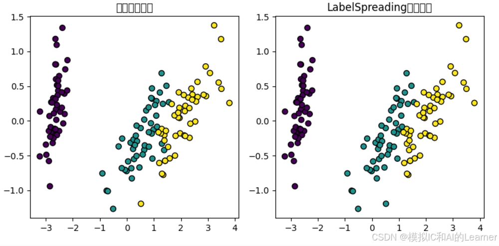
# 可选:可视化数据分布与传播结果(降维至二维)
from sklearn.decomposition import PCA
pca = PCA(n_components=2)
X_reduced = pca.fit_transform(X)
plt.figure(figsize=(8, 4))
plt.subplot(1, 2, 1)
plt.title("原始真实标签")
plt.scatter(X_reduced[:, 0], X_reduced[:, 1], c=y_true, cmap='viridis', edgecolor='k', s=40)
plt.subplot(1, 2, 2)
plt.title("LabelSpreading传播结果")
plt.scatter(X_reduced[:, 0], X_reduced[:, 1], c=y_pred, cmap='viridis', edgecolor='k', s=40)
plt.tight_layout()
plt.show()
总样本数: 150
有标签样本数量: 70
无标记样本位置: [ 0 4 5 6 10 13 14 15 16 18 19 21 22 23 24 26 29 31 32 36 37 39 40 41 42 44 46 49 56 57 58 59 60 61 63 64 66 68 71 72 77 78 79 82 83 84 85 89 90 95 97 98 99 100 102 105 106 108 109 110 111 117 122 123 124 125 128 130 131 132 133 135 138 141 142 143 144 145 148 149]
无标记样本数: 80
无标签样本上的准确率: 0.9625


 被折叠的 条评论
为什么被折叠?
被折叠的 条评论
为什么被折叠?
 到【灌水乐园】发言


