多项式插值（数值计算方法）Python实现

一. 原理介绍

1. 关于插值的定义及基本原理可以参照如下索引
   插值原理（数值计算方法）
2. 前面已经介绍过插值原理的唯一性表述，对于分立的数据点，方程组：

$$\begin{array}{rl}& P(x_0)=y_0\Rightarrow a_0+a_1{x}_0+a_2{x}_0^2+\cdots +a_n{x}_0^n=y_0,\\ & P(x_1)=y_1\Rightarrow a_0+a_1{x}_1+a_2{x}_1^2+\cdots +a_n{x}_1^n=y_1,\\ & ⋮\\ & P(x_n)=y_n\Rightarrow a_0+a_1{x}_n+a_2{x}_n^2+\cdots +a_n{x}_n^n=y_n.\end{array}$$

恒有解，多项式插值的目标即为在这一过程中求解系数$$a_0、a_1、...、a_n⟺\left[\begin{array}{c}{a}_0\\ a_1\\ a_2\\ ⋮\\ a_n\end{array}\right]$$

3. 即解方程组：
   $$\left[\begin{array}{ccccc}1& x_0& x_0^2& \cdots & x_0^n\\ 1& x_1& x_1^2& \cdots & x_1^n\\ ⋮& ⋮& ⋮& \ddots & ⋮\\ 1& x_n& x_n^2& \cdots & x_n^n\end{array}\right]\left[\begin{array}{c}{a}_0\\ a_1\\ a_2\\ ⋮\\ a_n\end{array}\right]=\left[\begin{array}{c}{y}_0\\ y_1\\ y_2\\ ⋮\\ y_n\end{array}\right].$$

关于该方程组的解法在线性代数中有多种，这里主要提及两种：
①高斯消元法
②克莱姆法则
程序设计过程中一般有封装好的库函数，如果为了考虑减少库依赖和提高程序运行效率及占用可能会用到上述方法（这里就不详细展开了）

---

二. 程序设计

1. 构建矩阵

A = np.zeros((n, n))
for i in range(n):
    for j in range(n):
        A[i, j] = x_data[i] ** j

Ⅰ 构建一个$(n\times n)$的矩阵 A 来描述多项式矩阵：
$$\left[\begin{array}{ccccc}1& x_0& x_0^2& \cdots & x_0^n\\ 1& x_1& x_1^2& \cdots & x_1^n\\ ⋮& ⋮& ⋮& \ddots & ⋮\\ 1& x_n& x_n^2& \cdots & x_n^n\end{array}\right]$$

其中：
$$A[i][j]=x_i^j$$

式中第一列的1是通过$x_i^0$得到的。

B = np.array(y_data)

Ⅱ 构建系数矩阵 B，即原始数据对应的 y 值：

2. 求解矩阵方程

coefficients = np.linalg.solve(A, B)

使用Numpy自带函数linalg.solve()解矩阵方程

注释：np.linalg.solve(A, B) 求解出的系数数组的顺序是 从低到高次项，即：

• coefficients[0] 为常数项（$x^0$ 的系数）
• coefficients[1] 为一次项（$x^1$ 的系数）
• coefficients[2] 为二次项（$x^2$ 的系数）
  以此类推。

求解出矩阵形式形如
[ 6. -7.83333333 4.5 -0.66666667]
从左至右为最低次项到最高次项系数

3. 作出多项式函数

x_data, y_data = zip(*data)

Ⅰ 获取输入数据（方法不唯一）

x_vals = np.linspace(min(x_data) - 1, max(x_data) + 1, 500)

Ⅱ 在数据点区间内构造间隔点来使绘图更加平滑（matplotlib.pyplot的局限性）

y_vals = np.polyval(coefficients[::-1], x_vals)

Ⅲ 通过Numpy内置函数np.polyval()来构造多项式函数(需要指定多项式系数)，实现输入 x 值，输出通过构造的多项式函数对应的函数值。

注释: 前面注释提到coefficients数组中的系数对应从左到右为最低到最高次项系数，而函数np.polyval()要求输入具有逆序的项系数：coefficients[::-1] 将变为从最高次到最低次项系数
np.polyval(coefficients[::-1], x_vals) 将计算每一个 x_val 对应的多项式值，并返回一个 y_vals 数组，包含每个 x_val 对应的 y 值。

4. 绘制插值曲线

	plt.rcParams['font.family'] = 'SimHei'
    plt.rcParams['axes.unicode_minus'] = False

通过替换显示字体('SimHei')和符号(False)来使图例正常显示中文和负号

    plt.plot(x_vals, y_vals, label="插值曲线", color='b')
    plt.scatter(x_data, y_data, color='r', label="数据点")
    plt.title("插值多项式")
    plt.xlabel("X轴")
    plt.ylabel("Y轴")
    plt.legend()
    plt.grid(True)
    plt.show()

5. 完整代码

import numpy as np
import matplotlib.pyplot as plt


def construct_interpolation_polynomial(data):
    # 提取x和y值
    x_data, y_data = zip(*data)
    n = len(data)

    # 构造矩阵A (n x n)
    A = np.zeros((n, n))

    # 构造矩阵A的每一列, A[i][j] = x_i^(j)
    for i in range(n):
        for j in range(n):
            A[i, j] = x_data[i] ** j

    # 构造常数向量B，B[i] = y_i
    B = np.array(y_data)

    # 解线性方程组 A * coefficients = B
    coefficients = np.linalg.solve(A, B)

    return coefficients


def plot_interpolation(data, coefficients):
    # 提取x和y值
    x_data, y_data = zip(*data)

    # 生成插值多项式的x和y值
    x_vals = np.linspace(min(x_data) - 1, max(x_data) + 1, 500)

    # 计算多项式的y值
    y_vals = np.polyval(coefficients[::-1], x_vals)

    # 绘图
    plt.rcParams['font.family'] = 'SimHei'
    plt.rcParams['axes.unicode_minus'] = False
    plt.plot(x_vals, y_vals, label="插值曲线", color='b')
    plt.scatter(x_data, y_data, color='r', label="数据点")
    plt.title("插值多项式")
    plt.xlabel("X轴")
    plt.ylabel("Y轴")
    plt.legend()
    plt.grid(True)
    plt.show()


# 定义输入数据 (xi, yi)
data = [
    [1, 2],
    [2, 3],
    [3, 5],
    [4, 4]
]

# 构造插值多项式的系数
coefficients = construct_interpolation_polynomial(data)

# 输出多项式的系数
print("插值多项式的系数:", coefficients)

# 绘制插值曲线
plot_interpolation(data, coefficients)

---

三. 图例

这要求我们的输入数据都具有上述形式：

data = [
    [x_1, y_1],
    [x_2, y_2],
    [x_3, y_3],
    [x_4, y_4],
    ...]

最后我们插值一组随机生成的测试数据

data = [
    [7.264384, 3.931292],
    [1.943873, 6.218903],
    [8.384019, 2.584103],
    [5.672210, 9.032674],
    [0.294315, 4.726018],
    [6.129531, 7.912846],
    [9.516347, 1.478264],
    [3.824679, 5.596042]
]

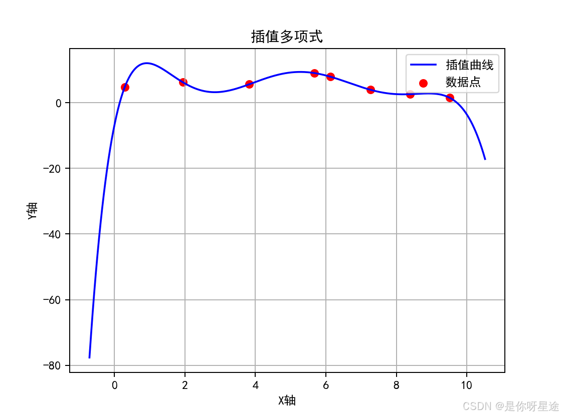
实际应用时应避免数据点过多导致的多项式次数过高

---

希望能够帮到迷途之中的你，知识有限，如有学术错误请及时指正，感谢大家的阅读

(^^)／▽ ▽＼(^^)