Regression Problems

Regression Problems

• Supervised learning：
  Given a data set that we already know the correct output is like, and want to discover the relationship between the input and the output.
  supervised learning is catagorized into “regression” and “classification” problems.

  • regression - function that generate continuous output
    • example：house price prediction
  • classification - classify the target into catagories which is a discrete output
    • example: classifying whether a tumor is malignant or benign

• Unsupervised learning:
  Given a data set that doesn’t have any labels or has the same label, and want to find some structure in the data.

  • clustering - group a large set of data into groups that is somehow similar or related by different variables or attributes.

    • examples:
      1. News grouping
      2. Market segmentation

  • non-clustering - find struction in a chaotic environment

    • examples:
      1. Cocktail party problem - cocktail party algorithm

Cost Function(Squared error function/Mean squared error):

$$J=\frac{1}{2m}\ast \sum _{i=1}^n(h_{\theta }(x^{(i)})-y^{(i)}{)}^2$$
Either devided by 2 * m or m results in the same thetas, while 2 * m used here is for convenience when taking derivative.
We can cut this function into two parts:
$$\begin{gathered} J({\theta }_0,{\theta }_1) \\ y(j)=h(x_j)={\theta }_0+thet{a}_1\ast x_j \end{gathered}$$
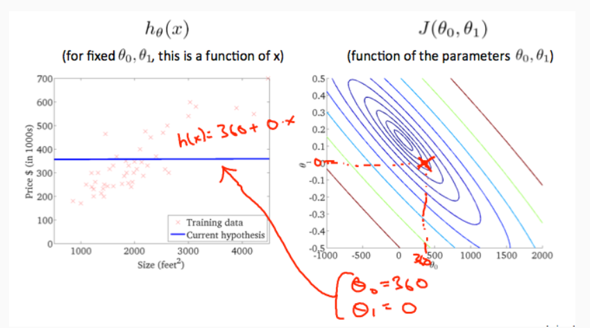
At first we can set $\theta$ to 0, and set $\theta$ to certain values and will get corresponding $h(x)$. Then we take the training set to the function to calculate $h(x_i)$ and then take the result into the function J and get a discrete $J(0,{\theta }_1)$, as plotted below:


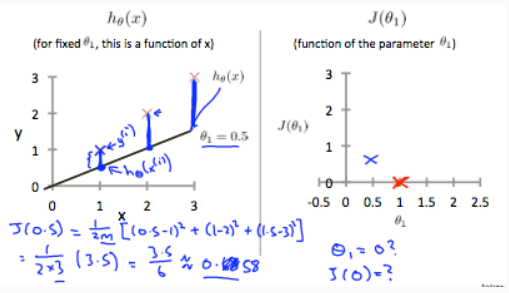
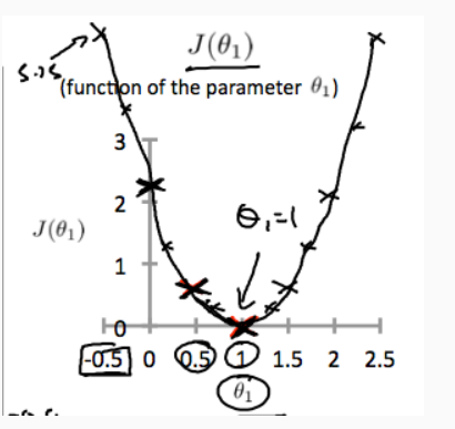
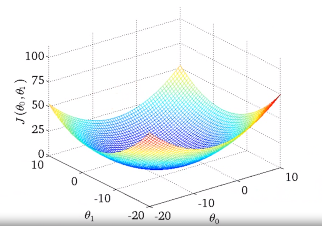
That’s when J is a univariable function. when ${\theta }_0$ comes in, the J function would be plotted like this:

And transfer it in a contour plot will be like this:

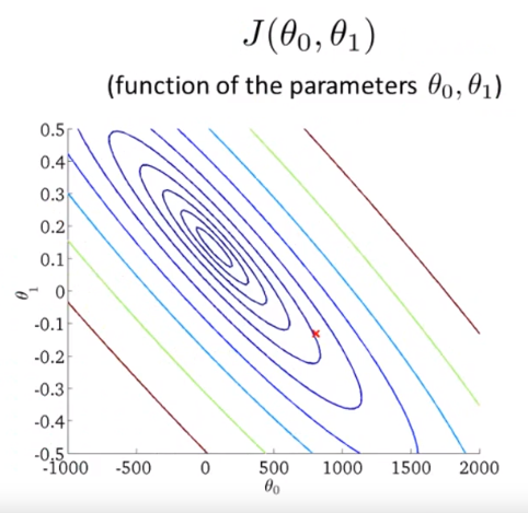
Plotting out our training set and select some fixed value for the two thetaes, we have hs of x. And we can point out the corresponding $J(\theta )$. matching the hs and the Js gives a clear version of the relationship of these two functions:

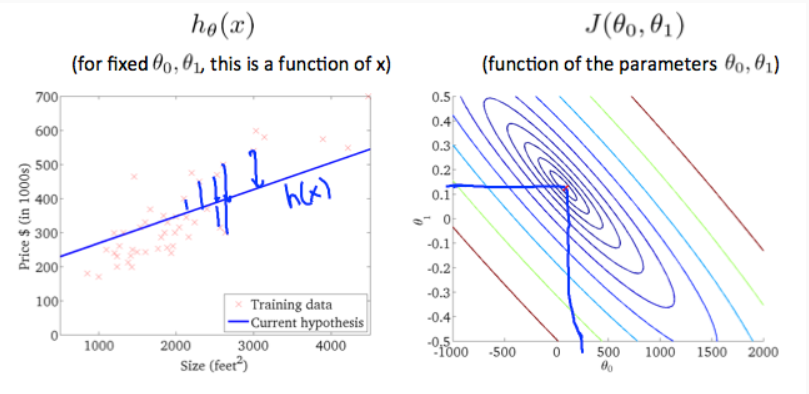
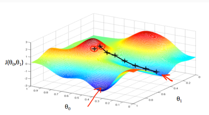
Gradient descent

To minimize all kinds of functions, we use gradient decent. when saying using gradient descent, we always mean that simultaneously subtract the variable.
As intuition in picture, we can say the descent comes as baby step as step walking down the hill, and finally reaching to the bottom of that route. If you start with another position on the hill, you would be reaching another bottom, while it might be real close to the first origin.

The algorithm is do the calculation repeatidly until convergence:
$${\theta }_i:={\theta }_i-\alpha \frac{\partial }{\partial {\theta }_i}J({\theta }_0,{\theta }_1,...)$$

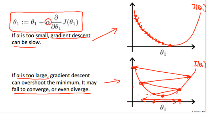
The alpha is called the learning rate, which means the step we take when updating parameters and it’s always a positive number. While i is the index number.

Pay attention to what we saying simultaneously update the parameters, it means that calculating each parameters prior to updating them. We shall do it this way:
$$\begin{gathered} \text{correct:} \\ tem{p}_0:={\theta }_0-\alpha \frac{\partial }{\partial {\theta }_0}J({\theta }_0...) \\ tem{p}_1:={\theta }_1-\alpha \frac{\partial }{\partial {\theta }_1}J({\theta }_0...) \\ ... \\ {\theta }_0=tem{p}_0 \\ {\theta }_1=tem{p}_1 \\ ... \end{gathered}$$
instead of doing it like this:
$$\begin{gathered} \text{Incorrect:} \\ tem{p}_0:={\theta }_0-\alpha \frac{\partial }{\partial {\theta }_0}J({\theta }_0...) \\ {\theta }_0=tem{p}_0 \\ tem{p}_1:={\theta }_1-\alpha \frac{\partial }{\partial {\theta }_1}J({\theta }_0...) \\ {\theta }_1=tem{p}_1 \\ ... \end{gathered}$$
In the algorithm, alpha controlls the rapidity that the parameter reaches the minimum. Either too small or too large is not appropriate. Too small will take it too many steps to the minimum which would cost a lot of time running the algorithm, while too large could overshot the minimum and may fail to convert or even divert.

Batch Gradient Descent:

Refers that in every step of gradient descent we’re looking at all the training examples. So when computing the derivatives, we’re computing the sums of each square error

There are other versions of gradient descent that look at small subsets of the training sets at a time.

（note：’:=’ means assignment same as ‘=’ in java, ‘=’ here means equalty same as ‘==’ in java

Version of Cost Function with Multiple Variable

Hypothesis with multiple variable:

Use n to denote the number of features and $x_n$ denotes the value of nth feature. with combination with superscript m, we get the nth parameter of mth training example:
$$\begin{gathered} x_j^{(i)}=\text{value of feature j in the }{i}^{th}\text{ training example} \\ {x}^{(i)}=\text{the input(features) of the }{i}^{th}\text{ training example} \end{gathered}$$
So the hypothesis function becomes like this:
$$h(\theta )={\theta }_0+{\theta }_1{x}_1+{\theta }_2{x}_2+...+{\theta }_n{x}_n$$
When we use vectors to describe, we assume there is a $x_0$ that equals 1, thus we get a vector that index from 0. assume $\overrightarrow{X}$ as a vector and parameters $\overrightarrow{\theta }$ as another vector, and we get two (n+1) by 1 vectors, and the function is like this:
$$h(\theta )=\left[\begin{array}{ccccc}{\theta }_0& {\theta }_1& {\theta }_2& ...& {\theta }_n\end{array}\right]\left[\begin{array}{c}{x}_1\\ x_1\\ x_2\\ ...\\ x_n\end{array}\right]$$
which is called multivariate linear regression.

Gradient Descent for multiple variables:

The gradient descent equation itself is generally the same form. We just have to repeat it for ‘n’ features:
repeat until convergence : { θ 0 : = θ 0 − α m ∑ i = 1 m ( h θ ( x ( i ) ) − y ( i ) ) ⋅ x 0 ( i ) θ 1 : = θ 1 − α m ∑ i = 1 m ( h θ ( x ( i ) ) − y ( i ) ) ⋅ x 1 ( i ) θ 2 : = θ 2 − α m ∑ i = 1 m ( h θ ( x ( i ) ) − y ( i ) ) ⋅ x 2 ( i ) . . . } \text{repeat until convergence}:\{\\ \theta_0 := \theta_0 - \frac{\alpha}{m}\sum_{i=1}^{m}(h_\theta(x^{(i)}) - y^{(i)})\cdot{x_0^{(i)}}\\ \theta_1 := \theta_1 - \frac{\alpha}{m}\sum_{i=1}^{m}(h_\theta(x^{(i)}) - y^{(i)})\cdot{x_1^{(i)}}\\ \theta_2 := \theta_2 - \frac{\alpha}{m}\sum_{i=1}^{m}(h_\theta(x^{(i)}) - y^{(i)})\cdot{x_2^{(i)}}\\ ...\\ \} repeat until convergence:{θ0​:=θ0​−mα​i=1∑m​(hθ​(x(i))−y(i))⋅x0(i)​θ1​:=θ1​−mα​i=1∑m​(hθ​(x(i))−y(i))⋅x1(i)​θ2​:=θ2​−mα​i=1∑m​(hθ​(x(i))−y(i))⋅x2(i)​...}
Or, in a compact form:
$${\theta }_j:={\theta }_j-\frac{\alpha }{m}\sum _{i=1}^n(h_{\theta }(x^{(i)}-y^{(i)}))\cdot x_j^{(i)}\text{ for j:= 0...n}$$

Feature Scaling and Mean Normalization:

It’s a trick to make the gradient descent more faster when u have features that range in different order of magnitude. Theta descend quickly on small ranges and slowly on large ranges, and so will oscillate inefficiently down to the optimum when the variables are very uneven.
The way to prevent this is to modify the ranges of our input variables so that they are all roughly the same. Ideally:
$$\begin{gathered} -1\le x_j\le 1 \\ or \\ -0.5\le x_j\le 0.5 \end{gathered}$$
Two techniques to help with this are feature scaling and mean normalization. Feature scaling involves dividing the input values by the range (i.e. the maximum value minus the minimum value) of the input variable, resulting in a new range of just 1. Mean normalization involves subtracting the average value for an input variable from the values for that input variable resulting in a new average value for the input variable of just zero. To implement both of these techniques, adjust your input values as shown in this formula:
$$x_j:=\frac{x_j-\mu }{s_j}$$

Practical Tips to Get Gradient Descent Working Correctly:

One way is to plot the cost function J of theta after each iteration. Our goal is to make sure the gradient descent would converge after iteration of algorithm. A pleasant iteration may look like this:

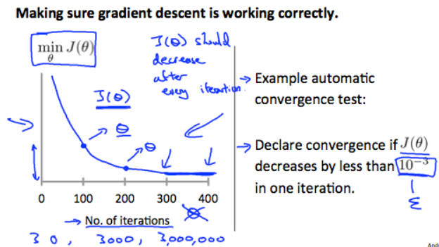
There are some common seen bug casing the plot unsatisfactory when doing iteration:

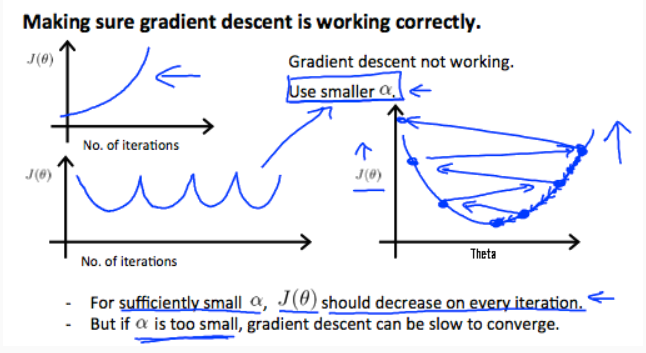
and they always cause by using large alpha, the learning rate. There’s a way for us to roughly get a workable alpha, which is to try out running gradient descent with a range of value of theta. Such as 0.001 and 0.01, and these different values of alpha plot J of theta as a function of number of iterations, and then pick the value of alpha that seems to be causing J to decrease rapidly. We can also increase the learning rate threefold to get 0.003, and so on.

Polynomial Regression:

We can improve our features and the form of the hypothesis function in a couple of different ways:
We can combine multiple features into one. For example, we can combine $x_1$ and $x_2$ into a new feature $x_3$ by taking $x_1\ast x_2$
Our hypothesis function need not to be linear when it doesn’t fit the data well. We can change the behavior of the curve of our hypothesis function by making it quadratic, cubic or square root function(or any other form).
For example, if we have a function like:
$$h(\theta )={\theta }_0+{\theta }_1{x}_1$$

Then we can create additional features based on x1 to get quadratic function:
$$h(\theta )={\theta }_0+{\theta }_1{x}_1+{\theta }_2{x}_1^2$$

or the cubic function:
$$h(\theta )={\theta }_0+{\theta }_1{x}_1+{\theta }_2{x}_1^2+{\theta }_3{x}_1^3$$

and we can create new features $x_2$, $x_3$ where $x_2=x_1^2$, $x_3=x_1^3$.
To make it a square root function, we could do:
$$h(\theta )={\theta }_0+{\theta }_1{x}_1+{\theta }_2\sqrt{x_1}$$

One important thing to keep in mind is that if we do this making our features 2 or 3 or more times, then feature scaling becomes very important. Cause if $x_1$ has range 1 - 1000, the $x_1$ square becomes 1 - 100000.

Normal Equation:

Instead of iterative method like gradient descent, we can solve for the optimal value for theta all at one go.
Without proving, just given the method to calculate the theta.
First we set X is a m by (n+1) matrix a combination of vectors of each training example, and y a m dimensional vector containing each known result. And then we get theta:
$$\theta =(X^{T}X{)}^{-1}{X}^{T}y$$

• Example: m=4

$x_0$	Size(feet)$x_1$	Number of bedrooms$x_2$	Number of floors$x_3$	Age of home(years)$x_4$	Price$1000$y
1	2104	5	1	45	460
1	1416	3	2	40	232
1	1534	3	2	30	315
1	852	2	1	36	178

$$\begin{gathered} X=\left[\begin{array}{ccccc}1& 2104& 5& 1& 45\\ 1& 1416& 3& 2& 40\\ 1& 1534& 3& 2& 30\\ 1& 852& 2& 1& 36\end{array}\right]y=\left[\begin{array}{c}460\\ 232\\ 315\\ 178\end{array}\right] \\ \theta =(X^{T}X{)}^{-1}{X}^{T}y \end{gathered}$$

There is no need to do features scaling when using normal equation. The following is a comparison of gradient descent and normal equation:

Gradient Descent	Normal Equation
need to choose alpha	no need to choose alpha
needs many iteration	no need to iterate
$O(k{n}^2)$	$O(n^3)$, need to calculate inverse of $X^{T}X$
works well with large n	slow if n is large

In addition, gradient descent still works for some classification problems while normal equation doesn’t.

Classification（binary classification/mutiple classification):

Logistic Regression:

The prediction is between 0 and 1:
$$0\le h_{\theta }(x)\le 1$$
which the output of h estimate the probability that y = 1 on input x

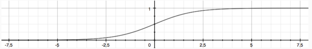
So we need a function to generate output only between 0 and 1. Thats when we found Sigmoid function/Logistic function to meet our need:
$$g(z)=\frac{1}{1+e^{-z}}$$

Sigmoid function can restrain the output beween 0 and 1, which look like this:

So we can take our hypothesis function into z, like:
$$\begin{gathered} h_{\theta }(x)=g({\theta }^{T}x) \\ z={\theta }^{T}x \end{gathered}$$

Descision boundary:

Suppose

• predict “y = 1” if the output is greater than or equal to 0.5
• predict “y = 0” if the output is less than 0.5

In other word, the boundary can be defined by parameterized $x$, whether it is greater or smaller than 0

The decision boundary is a property, not of the trading set, but of the hypothesis under the parameters. So, so long as we’re given my parameter vector theta, that defines the decision boundary. But the training set is not what we use to define the decision boundary. The training set may be used to fit the parameters $\theta$.

The hypothesis doesn’t need to be linear, and could be a function that describes a circle like:
$$(e.g.z={\theta }_0+{\theta }_1{x}_1^2+{\theta }_2{x}_2^3)$$
or any shape to fit our data.

Logistic regression cost funciton:

Using the same cost function as linear regression may cause multiple local optima, plotting a wavy or we say non-convex figure. So we have to find a better cost function:
$$\begin{gathered} J(\theta )=\frac{1}{m}\sum _{i=1}^m\text{Cost}(h_{\theta }(x^{(i)},y^{(i)}) \\ \text{Cost}(h_{\theta }(x),y)=-log(h_{\theta }(x^{(i)})) \end{gathered}$$
Writing the cost function in this way guarantees that J of theta is convex for logistic regression.
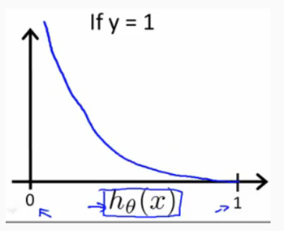
When y = 1, we get the following plot for J of theta vs H of theta:

Similarly, when y = 0:

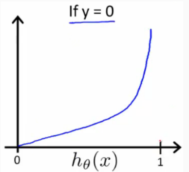
Whether the y is 0 or 1, if our hypothesis reach the other side of y, the cost function would approach infinity:
$$\begin{gathered} Cost(h_{\theta }(x),y)=0\text{if}{h}_{\theta }(x)=y \\ Cost(h_{\theta }(x),y)\to \infty \text{if}y=0\text{and}{h}_{\theta }(x)\to 1 \\ Cost(h_{\theta }(x),y)\to \infty \text{if}y=1\text{and}{h}_{\theta }(x)\to 0 \end{gathered}$$
To make the cost function simpler, we can combine the two condition together adding a coeffecient of treated y:
$$y^{(i)}\ln h_{\theta }(x^{(i)})+(1-y^{(i)})\ln (1-h_{\theta }(x^{(i)}))$$
So the J of theta would end up looking like this:
$$\begin{gathered} J(\theta )=\frac{1}{m}\sum _{i=1}^{m}Cost(h_{\theta }(x^{(i)},y) \\ =-\frac{1}{m}[\sum _{i=1}^m{y}^{(i)}\ln h_{\theta }(x^{(i)})+(1-y^{(i)})\ln (1-h_{\theta }(x^{(i)}))] \end{gathered}$$
And the gradient descent algorithm is identical to the one we used in linear regression, while h’s in the two functions are different:
R e p e a t : { θ j = θ j − α ∂ ∂ θ j J ( θ ) } Repeat:\{\\ \theta_j = \theta_j - \alpha\frac{\partial}{\partial\theta_j}J(\theta)\\ \} Repeat:{θj​=θj​−α∂θj​∂​J(θ)}

After working out the derivative part to get:
R e p e a t : { θ j = θ j − α m ∑ i = 1 m ( h θ ( x ( i ) ) − y ( i ) ) x j ( i ) } Repeat:\{\\ \theta_j = \theta_j - \frac{\alpha}{m}\sum_{i=1}^m(h_\theta(x^{(i)}) - y^{(i)})x_j^{(i)}\\ \} Repeat:{θj​=θj​−mα​i=1∑m​(hθ​(x(i))−y(i))xj(i)​}
A vectorized implementation is:
$$\begin{gathered} h=g(X\theta ) \\ J(\theta )=\frac{1}{m}\cdot (-y^T\ln (h)-(1-y{)}^T\ln (1-h)) \end{gathered}$$

Note that feature scaling also work for logistic regression.

Advanced Optimization Algorithm:

There are more safisticated algorithms given by experts to calculate the optimal theta:

• Conjugate gradient
• BFGS
• L-BFGS

The advantage of using these is that they’re much more faster than just simply applying gradient descent, mostly because that they could choose a more suitable learning rate during iteration, some of them can even choose better alpha for each iteration.
The disadvange is that they’re more complicate. It’s not easy for us to really figure out what they’re doing in the inner loop, unless we have expertise upon the area.
To apply these in octave, we first have to write a costFunction() ourselves returning a J of theta, and a vector containing each gradient of thetaes:

function [jVal, gradient] = costFunction(theta)

jVal = [code to compute J(theta)];

gradient(1) = [code to compute J(theta) partial to theta1]

...

gradient(n)  = [code to compute J(theta) partial to thetan]

Then call two built-in functions to make the advanced optimized algorithm works:

Multiclass Classification:

The main idea of multiclass classification is seperating each set of data from other. Similar with binary classification, we’ll have cost funtion. What’s different is that we’ll calculate each cost function for each sort of data. In practice, we basically choose one class and then lump all the others into a single second class. Then do this repeatedly, apply binary logistic regression to each case, and use the hypothesis that returned the highest value as our prediction:
y ∈ { 0 , 1 , 2 , . . . , n } h θ ( 0 ) ( x ) = P ( y = 0 ∣ x ; θ ) h θ ( 1 ) ( x ) = P ( y = 1 ∣ x ; θ ) . . . h θ ( n ) ( x ) = P ( y = n ∣ x ; θ ) prediction = max ⁡ ( h θ ( i ) ( x ) ) y \in \{0, 1, 2, ..., n\}\\ h_\theta ^{(0)}(x) = P(y = 0\mid x; \theta)\\ h_\theta ^{(1)}(x) = P(y = 1\mid x; \theta)\\ ...\\ h_\theta ^{(n)}(x) = P(y = n\mid x; \theta)\\ \text{prediction} = \max(h_\theta ^{(i)}(x)) y∈{0,1,2,...,n}hθ(0)​(x)=P(y=0∣x;θ)hθ(1)​(x)=P(y=1∣x;θ)...hθ(n)​(x)=P(y=n∣x;θ)prediction=max(hθ(i)​(x))
To summarize, after we train out each classifier, we take the x to predict into every cost function and pick the class that maximizes h.

Underfitting and Overfitting:

When fitting the data, we may encounter these kinds of problem:

• underfitting: when the power of our hypothesis function is too small. For instance, we fit a quadratic model of data with a straight line, the data won’t fit the line well:

• overfitting: when the power we set to our hypothesis function is too large, or when we add too many features, we may get a line fit almost every given data perfectly. But it doesn’t mean the prediction works well.

To deal with overfitting, we have two options:

• Reduce the number of features:
  • Manually select which features to keep
  • Use a model selection algorithm
• Regularization:
  • Keep all the features, but reduce the magnitude of parameter theta j

Regularization works well when we have a lot of slightly useful features

Regularization:

Penalize some of the thetaes to make them smaller would cause:

• simpler hypothesis
• less prone to overfitting

If we have overfitting problem, we can reduce the weight that some of the terms if our function carry by increasing their cost.
Say if we wanted to make the following function more quadratic:
$${\theta }_0+{\theta }_{1}x+{\theta }_2{x}^2+{\theta }_3{x}^3+{\theta }_4{x}^4$$
We’ll want to eliminate the influence of ${\theta }_3{x}^3$ and ${\theta }_4{x}^4$ . Without actually getting rid of these features or changing the form of our hypothesis, we can instead modify our cost function:
$$\underset{\theta }{\min }\frac{1}{m}\sum _{i=1}^m(h_{\theta }(x^{(i)})-y^{(i)}{)}^2+1000\cdot {\theta }_3^2+1000\cdot {\theta }_4^2$$
We’ve added two extra terms at the end to inflate the cost of ${\theta }_3$ and ${\theta }_4$. Now, in order for the cost function to get close to zero, we will have to reduce the values of ${\theta }_3$ and ${\theta }_4$ to near zero. This will in turn greatly reduce the values of ${\theta }_3$ and ${\theta }_4$ in our hypothesis function. As a result, we see that the new hypothesis (depicted by the pink curve) looks like a quadratic function but fits the data better due to the extra small terms ${\theta }_3{x}^3$ and ${\theta }_4{x}^4$.
To generallize, we make our cost function like this:
$$\underset{\theta }{\min }\frac{1}{m}\sum _{i=1}^m(h_{\theta }(x^{(i)})-y^{(i)}{)}^2+\lambda \sum _{j=1}^n{\theta }_j^2$$

while the $\lambda$ is the regularization parameter.

Gradient descent:

when doing gradient descent, the thetaes will have to subtract the extra part:
Repeat: { θ 0 : = θ 0 − α m ∑ i = 1 m ( h θ ( x ( i ) ) − y ( i ) ) x 0 ( i ) θ j : = θ j − α m ∑ i = 1 m ( h θ ( x ( i ) ) − y ( i ) ) x j ( i ) + α λ m θ j ) } θ j : = ( 1 − α m ) θ j − α m ∑ i = 1 m ( h θ ( x ( i ) ) − y ( i ) ) x j ( i ) ,    j = ( 1 , 2 , 3 , 4 , . . . , n )  without 0 \text{Repeat:}\{\\ \theta_0 := \theta_0 - \frac{\alpha}{m}\sum_{i=1}^m (h_\theta(x^{(i)}) - y^{(i)})x_0^{(i)}\\ \theta_j := \theta_j - \frac{\alpha}{m}\sum_{i=1}^m (h_\theta(x^{(i)}) - y^{(i)})x_j^{(i)} + \frac{\alpha\lambda}{m}\theta_j)\\ \}\\ \large{\theta_j} := (1 - \frac{\alpha}{m})\theta_j - \frac{\alpha}{m}\sum_{i=1}^m (h_\theta(x^{(i)}) - y^{(i)})x_j^{(i)}, \space\space j = (1, 2, 3, 4, ..., n)\space\text{without 0} Repeat:{θ0​:=θ0​−mα​i=1∑m​(hθ​(x(i))−y(i))x0(i)​θj​:=θj​−mα​i=1∑m​(hθ​(x(i))−y(i))xj(i)​+mαλ​θj​)}θj​:=(1−mα​)θj​−mα​i=1∑m​(hθ​(x(i))−y(i))xj(i)​,  j=(1,2,3,4,...,n) without 0

which is exactly the same as what gradient descent was doing before, just a little bit of difference of appearance.
Notice the $(1-\frac{\alpha }{m})$ is going to be a little bit smaller than 1

Normal equation:

$$\begin{gathered} \theta =(X^{T}X+\lambda \cdot L{)}^{-1}{X}^{T}y \\ whereL=\left[\begin{array}{cccccc}0& & & & & \\ & 1& & & & \\ & & 1& & & \\ & & & .& & \\ & & & & .& \\ & & & & & 1\end{array}\right] \end{gathered}$$

Regularized logistic regression:

Recall the cost function of the logistic regression was:
$$J(\theta )=-\frac{1}{m}\sum _{i=1}^m[y^{(i)}\ln (h_{\theta }(x^{(i)}))+(1-y^{(i)})\ln (1-h_{\theta }(x^{(i)}))]$$
We can regularize this equation by adding a term to the end:
$$J(\theta )=-\frac{1}{m}\sum _{i=1}^m[y^{(i)}\ln (h_{\theta }(x^{(i)}))+(1-y^{(i)})\ln (1-h_{\theta }(x^{(i)}))]+\frac{\lambda }{2m}\sum _{j=1}^n{\theta }_j^2$$
The second sum exclude ${\theta }_0$. But when we compute it as a vector, we should take ${\theta }_0$ into account. We should continuously update the two following equations:
Repeat: { θ 0 : = θ 0 − α m ∑ i = 1 m ( h θ ( x ( i ) ) − y ( i ) ) x 0 ( i ) θ j : = θ j − α m ∑ i = 1 m ( h θ ( x ( i ) ) − y ( i ) ) x j ( i ) + α λ m θ j } \text{Repeat:}\{\\ \theta_0 := \theta_0 - \frac{\alpha}{m}\sum_{i=1}^m (h_\theta(x^{(i)}) - y^{(i)})x_0^{(i)}\\ \theta_j := \theta_j - \frac{\alpha}{m}\sum_{i=1}^m (h_\theta(x^{(i)}) - y^{(i)})x_j^{(i)} + \frac{\alpha\lambda}{m}\theta_j\\ \} Repeat:{θ0​:=θ0​−mα​i=1∑m​(hθ​(x(i))−y(i))x0(i)​θj​:=θj​−mα​i=1∑m​(hθ​(x(i))−y(i))xj(i)​+mαλ​θj​}