


1. 导入库 筛选离散特征 对离散特征进行标签编码 独热编码 以及缺失值的中位数补全
import pandas as pd
import pandas as pd    #用于数据处理和分析,可处理表格数据。
import numpy as np     #用于数值计算,提供了高效的数组操作。
import matplotlib.pyplot as plt    #用于绘制各种类型的图表
import seaborn as sns   #基于matplotlib的高级绘图库,能绘制更美观的统计图形。

 # 设置中文字体(解决中文显示问题)
plt.rcParams['font.sans-serif'] = ['SimHei']  # Windows系统常用黑体字体
plt.rcParams['axes.unicode_minus'] = False    # 正常显示负号
data = pd.read_csv('data.csv')    #读取数据

# 先筛选字符串变量
discrete_features = data.select_dtypes(include=['object']).columns.tolist()
# Home Ownership 标签编码
home_ownership_mapping = {
    'Own Home': 1,
    'Rent': 2,
    'Have Mortgage': 3,
    'Home Mortgage': 4
}
data['Home Ownership'] = data['Home Ownership'].map(home_ownership_mapping)

# Years in current job 标签编码
years_in_job_mapping = {
    '< 1 year': 1,
    '1 year': 2,
    '2 years': 3,
    '3 years': 4,
    '4 years': 5,
    '5 years': 6,
    '6 years': 7,
    '7 years': 8,
    '8 years': 9,
    '9 years': 10,
    '10+ years': 11
}
data['Years in current job'] = data['Years in current job'].map(years_in_job_mapping)

# Purpose 独热编码,记得需要将bool类型转换为数值
data = pd.get_dummies(data, columns=['Purpose'])
data2 = pd.read_csv("data.csv") # 重新读取数据,用来做列名对比
list_final = [] # 新建一个空列表,用于存放独热编码后新增的特征名
for i in data.columns:
    if i not in data2.columns:
       list_final.append(i) # 这里打印出来的就是独热编码后的特征名
for i in list_final:
    data[i] = data[i].astype(int) # 这里的i就是独热编码后的特征名


# Term 0 - 1 映射
term_mapping = {
    'Short Term': 0,
    'Long Term': 1
}
data['Term'] = data['Term'].map(term_mapping)
data.rename(columns={'Term': 'Long Term'}, inplace=True) # 重命名列
continuous_features = data.select_dtypes(include=['int64', 'float64']).columns.tolist()  #把筛选出来的列名转换成列表

 # 连续特征用中位数补全
for feature in continuous_features:
    mode_value = data[feature].mode()[0]            #获取该列的众数。
    data[feature].fillna(mode_value, inplace=True)          #用众数填充该列的缺失值,inplace=True表示直接在原数据上修改。
purpose独热编码的具体理解 前几天没搞懂
- 使用
pd.get_dummies对'Purpose'列进行独热编码,将分类特征转换为机器学习模型可以理解的二元数值特征。 - 读取一个原始的 CSV 文件到
data2,用于对比。 - 找出所有在经过独热编码后的
dataDataFrame 中存在,但在原始data2DataFrame 中不存在的列。这些通常是新生成的独热编码列。 - 将这些新生成的独热编码列的数据类型强制转换为整数(0和1),以确保它们是干净的数值类型,方便后续的建模。
2.划分训练集 验证集 测试集的方法
from sklearn.model_selection import train_test_split
X = data.drop(['Credit Default'], axis=1)  # 特征,axis=1表示按列删除
y = data['Credit Default']  # 标签
# 按照8:1:1划分训练集、验证集和测试集
X_train, X_temp, y_train, y_temp = train_test_split(X, y, test_size=0.2, random_state=42)  # 80%训练集,20%临时集
X_val, X_test, y_val, y_test = train_test_split(X_temp, y_temp, test_size=0.5, random_state=42)  # 50%验证集,50%测试集

print("Data shapes:")
print("X_train:", X_train.shape)
print("y_train:", y_train.shape)
print("X_val:", X_val.shape)
print("y_val:", y_val.shape)
print("X_test:", X_test.shape)
print("y_test:", y_test.shape) 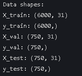
可以看见val 和test 均占10%
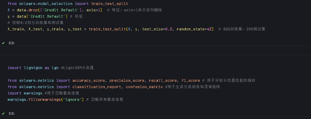
3.由于许多函数自带交叉验证 所以如果想不交叉比较麻烦 只需划分一次训练集与测试集
from sklearn.model_selection import train_test_split
X = data.drop(['Credit Default'], axis=1)  # 特征,axis=1表示按列删除
y = data['Credit Default'] # 标签
# 按照8:2划分训练集和测试集
X_train, X_test, y_train, y_test = train_test_split(X, y, test_size=0.2, random_state=42)  # 80%训练集,20%测试集
4. 导入随机森林并进行调参
from sklearn.ensemble import RandomForestClassifier #随机森林分类器

from sklearn.metrics import accuracy_score, precision_score, recall_score, f1_score # 用于评估分类器性能的指标
from sklearn.metrics import classification_report, confusion_matrix #用于生成分类报告和混淆矩阵
import warnings #用于忽略警告信息
warnings.filterwarnings("ignore") # 忽略所有警告信息
默认参数
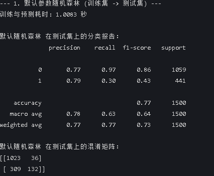
print("--- 1. 默认参数随机森林 (训练集 -> 测试集) ---")
import time # 这里介绍一个新的库,time库,主要用于时间相关的操作,因为调参需要很长时间,记录下会帮助后人知道大概的时长
start_time = time.time() # 记录开始时间
rf_model = RandomForestClassifier(random_state=42)
rf_model.fit(X_train, y_train) # 在训练集上训练
rf_pred = rf_model.predict(X_test) # 在测试集上预测
end_time = time.time() # 记录结束时间

print(f"训练与预测耗时: {end_time - start_time:.4f} 秒")
print("\n默认随机森林 在测试集上的分类报告:")
print(classification_report(y_test, rf_pred))
print("默认随机森林 在测试集上的混淆矩阵:")
print(confusion_matrix(y_test, rf_pred))
这里time函数用于计时import time
start_time = time.time()
end_time = time.time()
网格搜索 找参数
print("\n--- 2. 网格搜索优化随机森林 (训练集 -> 测试集) ---")
from sklearn.model_selection import GridSearchCV

# 定义要搜索的参数网格
param_grid = {
    'n_estimators': [50, 100, 200],
    'max_depth': [None, 10, 20, 30],
    'min_samples_split': [2, 5, 10],
    'min_samples_leaf': [1, 2, 4]
}

# 创建网格搜索对象
grid_search = GridSearchCV(estimator=RandomForestClassifier(random_state=42), # 随机森林分类器
                           param_grid=param_grid, # 参数网格
                           cv=5, # 5折交叉验证
                           n_jobs=-1, # 使用所有可用的CPU核心进行并行计算
                           scoring='accuracy') # 使用准确率作为评分标准

start_time = time.time()
# 在训练集上进行网格搜索
grid_search.fit(X_train, y_train) # 在训练集上训练,模型实例化和训练的方法都被封装在这个网格搜索对象里了
end_time = time.time()

print(f"网格搜索耗时: {end_time - start_time:.4f} 秒")
print("最佳参数: ", grid_search.best_params_) #best_params_属性返回最佳参数组合

# 使用最佳参数的模型进行预测
best_model = grid_search.best_estimator_ # 获取最佳模型
best_pred = best_model.predict(X_test) # 在测试集上进行预测

print("\n网格搜索优化后的随机森林 在测试集上的分类报告:")
print(classification_report(y_test, best_pred))
print("网格搜索优化后的随机森林 在测试集上的混淆矩阵:")
print(confusion_matrix(y_test, best_pred))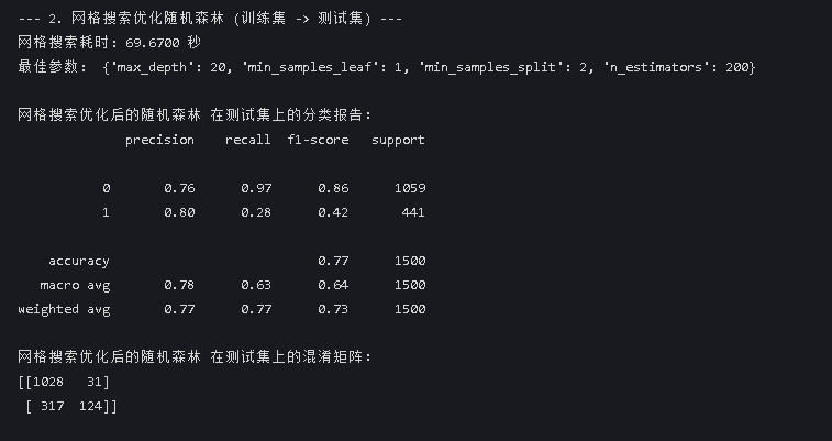
贝叶斯优化
print("\n--- 2. 贝叶斯优化随机森林 (训练集 -> 测试集) ---")
from skopt import BayesSearchCV
from skopt.space import Integer
from sklearn.ensemble import RandomForestClassifier
from sklearn.metrics import classification_report, confusion_matrix
import time

# 定义要搜索的参数空间
search_space = {
    'n_estimators': Integer(50, 200),
    'max_depth': Integer(10, 30),
    'min_samples_split': Integer(2, 10),
    'min_samples_leaf': Integer(1, 4)
}

# 创建贝叶斯优化搜索对象
bayes_search = BayesSearchCV(
    estimator=RandomForestClassifier(random_state=42),
    search_spaces=search_space,
    n_iter=32,  # 迭代次数,可根据需要调整
    cv=5, # 5折交叉验证,这个参数是必须的,不能设置为1,否则就是在训练集上做预测了
    n_jobs=-1,
    scoring='accuracy'
)

start_time = time.time()
# 在训练集上进行贝叶斯优化搜索
bayes_search.fit(X_train, y_train)
end_time = time.time()

print(f"贝叶斯优化耗时: {end_time - start_time:.4f} 秒")
print("最佳参数: ", bayes_search.best_params_)

# 使用最佳参数的模型进行预测
best_model = bayes_search.best_estimator_
best_pred = best_model.predict(X_test)

print("\n贝叶斯优化后的随机森林 在测试集上的分类报告:")
print(classification_report(y_test, best_pred))
print("贝叶斯优化后的随机森林 在测试集上的混淆矩阵:")
print(confusion_matrix(y_test, best_pred)) 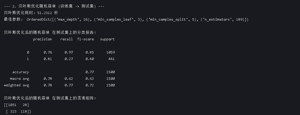
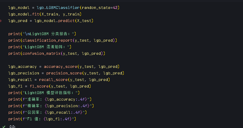
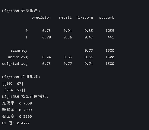
5.针对lightgbm自己试着进行调参
网格搜索
print("\n--- 2. 网格搜索优化lightgbm (训练集 -> 测试集) ---")
from sklearn.model_selection import GridSearchCV
import time
# 定义要搜索的参数网格
param_grid = {
    'n_estimators': [50, 100, 200], # 树的数量
   'max_depth': [None, 10, 20, 30], # 树的最大深度
   'learning_rate': [0.01, 0.1, 0.2], # 学习率
}

# 创建网格搜索对象
grid_search = GridSearchCV(estimator=lgb.LGBMClassifier(random_state=42), # 随机森林分类器
                           param_grid=param_grid, # 参数网格
                           cv=5, # 5折交叉验证
                           n_jobs=-1, # 使用所有可用的CPU核心进行并行计算
                           scoring='accuracy') # 使用准确率作为评分标准

start_time = time.time()
# 在训练集上进行网格搜索
grid_search.fit(X_train, y_train) # 在训练集上训练,模型实例化和训练的方法都被封装在这个网格搜索对象里了
end_time = time.time()

print(f"网格搜索耗时: {end_time - start_time:.4f} 秒")
print("最佳参数: ", grid_search.best_params_) #best_params_属性返回最佳参数组合

# 使用最佳参数的模型进行预测
best_model = grid_search.best_estimator_ # 获取最佳模型
best_pred = best_model.predict(X_test) # 在测试集上进行预测

print("\n网格搜索优化后的lightgbm 在测试集上的分类报告:")
print(classification_report(y_test, best_pred))
print("网格搜索优化后的lightgbm 在测试集上的混淆矩阵:")

print(confusion_matrix(y_test, best_pred))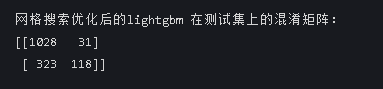
贝叶斯优化
print("\n--- 3.贝叶斯优化LightGBM (训练集 -> 测试集) ---")
from bayes_opt import BayesianOptimization #用于贝叶斯优化
from skopt import BayesSearchCV #用于贝叶斯优化
from skopt.space import Integer, Real #用于贝叶斯优化
# 定义要搜索的参数空间
search_space = {
    'n_estimators': Integer(50, 200), # 树的数量
   'max_depth': Integer(10, 30), # 树的最大深度
   'learning_rate': Real(0.01, 0.2), # 学习率
}
# 创建贝叶斯优化对象
bayes_search = BayesSearchCV(estimator=lgb.LGBMClassifier(random_state=42), # 创建LightGBM分类器
                             search_spaces=search_space, # 参数空间
                             cv=5, # 交叉验证折数
                             scoring='accuracy', # 使用准确率作为评估指标
                             n_iter=32, # 迭代次数
                             n_jobs=-1) # 使用所有可用的CPU核心进行并行计算
# 开始贝叶斯优化
start_time = time.time() # 记录开始时间
bayes_search.fit(X_train, y_train) # 训练模型
end_time = time.time() # 记录结束时间
# 输出最佳参数和最佳得分
print(f"贝叶斯优化耗时: {end_time - start_time:.4f} 秒")
print(f"最佳参数: {bayes_search.best_params_}") # 打印最佳参数
# 使用最佳参数的模型进行预测
best_lgb = bayes_search.best_estimator_ # 获取最佳模型
best_lgb_pred = best_lgb.predict(X_test) # 预测测试集
# 计算并打印评估指标
print("\n贝叶斯优化后的LightGBM在测试集上的分类报告:")
print(classification_report(y_test, best_lgb_pred)) # 打印分类报告
print("贝叶斯优化后的LightGBM在测试集上的混淆矩阵:")
print(confusion_matrix(y_test, best_lgb_pred)) # 打印混淆矩阵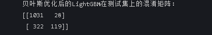


 1671
1671

 被折叠的 条评论
为什么被折叠?
被折叠的 条评论
为什么被折叠?
 到【灌水乐园】发言


