Python自动控制（三）

原创于 2022-08-25 20:58:29 发布 · 537 阅读

0 ·

CC 4.0 BY-SA版权

文章标签：

#python #自动化

Python 专栏收录该内容

4 篇文章

订阅专栏

本文探讨了Python在实现二自由度控制中的应用，重点讲解了PI-D和I-PD控制器的设计与实现，为自动化控制提供了解决方案。

部署运行你感兴趣的模型镜像

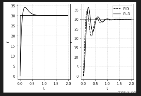
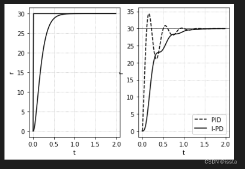
二自由度之PI-D与I-PD控制

import control as ctrl
from control.matlab import *
import sympy as sp
import matplotlib.pyplot as plt
import numpy as np

#--------------------------------------------------------
def linestyle_generator():
    linestyle = ['-', '--', '-.', ':']
    lineID = 0
    while True:
        yield linestyle[lineID]
        lineID = (lineID + 1) % len(linestyle)

def plot_set(fig_ax, *argv):
    fig_ax.set_xlabel(argv[0])
    fig_ax.set_ylabel(argv[1])

    fig_ax.grid(ls=':')
    if len(argv) == 3:
        fig_ax.legend(loc=argv[2])

def bodeplot_set(fig_ax, *argv):
    fig_ax[0].grid(which='both', ls=':')
    fig_ax[0].set_ylabel('Gain [dB')

    fig_ax[1].grid(which='both', ls=':')
    fig_ax[1].set_xlabel('$\omega$ [rad/s]')
    fig_ax[1].set_ylabel('Phase [deg')

    if len(argv) > 0:
        fig_ax[1].legend(loc=argv[0])
    if len(argv) > 1:
        fig_ax[0].legend(loc=argv[1])
#--------------------------------------------------------

g = 9.81 
L = 0.2
M = 0.5
mu = 1.5e-2
J = 1.0e-2

P = ctrl.tf([0, 1], [J, mu, M*g*L])
ref = 30

#--------------------------------------------------------

kp = 2
ki = 10
kd = 0.1

K1 = ctrl.tf([kd, kp, ki], [1, 0])
K2 = ctrl.tf([kp, ki], [kd, kp, ki])

Gyz = ctrl.feedback(P * K1, 1)
Td = np.arange(0, 2, 0.01)
r = 1 * (Td > 0)

z, t, _ = lsim(K2, r, Td, 0)
z, t, _ = lsim(K3, r, Td, 0)
fig, ax = plt.subplots(1, 2)

y, _, _ = lsim(Gyz, r, Td, 0)
ax[0].plot(t, r*ref, color='k')
ax[1].plot(t, y*ref, ls='--', label='PID', color='k')

y, _, _ = lsim(Gyz, z, Td, 0)
ax[0].plot(t, z*ref, color='k')
ax[1].plot(t, y*ref, label='PI-D', color='k')

ax[1].axhline(ref, color='k', linewidth=0.5)
plot_set(ax[0], 't', 'r')
plot_set(ax[1], 't', 'r', 'best')

import control as ctrl
from control.matlab import *
import sympy as sp
import matplotlib.pyplot as plt
import numpy as np

#--------------------------------------------------------
def linestyle_generator():
    linestyle = ['-', '--', '-.', ':']
    lineID = 0
    while True:
        yield linestyle[lineID]
        lineID = (lineID + 1) % len(linestyle)

def plot_set(fig_ax, *argv):
    fig_ax.set_xlabel(argv[0])
    fig_ax.set_ylabel(argv[1])

    fig_ax.grid(ls=':')
    if len(argv) == 3:
        fig_ax.legend(loc=argv[2])

def bodeplot_set(fig_ax, *argv):
    fig_ax[0].grid(which='both', ls=':')
    fig_ax[0].set_ylabel('Gain [dB')

    fig_ax[1].grid(which='both', ls=':')
    fig_ax[1].set_xlabel('$\omega$ [rad/s]')
    fig_ax[1].set_ylabel('Phase [deg')

    if len(argv) > 0:
        fig_ax[1].legend(loc=argv[0])
    if len(argv) > 1:
        fig_ax[0].legend(loc=argv[1])
#--------------------------------------------------------

g = 9.81 
L = 0.2
M = 0.5
mu = 1.5e-2
J = 1.0e-2

P = ctrl.tf([0, 1], [J, mu, M*g*L])
ref = 30

#--------------------------------------------------------

kp = 2
ki = 10
kd = 0.1

K1 = ctrl.tf([kd, kp, ki], [1, 0])
K3 = ctrl.tf([0, ki], [kd, kp, ki])

Gyz = ctrl.feedback(P * K1, 1)
Td = np.arange(0, 2, 0.01)
r = 1 * (Td > 0)

z, t, _ = lsim(K3, r, Td, 0)
fig, ax = plt.subplots(1, 2)

y, _, _ = lsim(Gyz, r, Td, 0)
ax[0].plot(t, r*ref, color='k')
ax[1].plot(t, y*ref, ls='--', label='PID', color='k')

y, _, _ = lsim(Gyz, z, Td, 0)
ax[0].plot(t, z*ref, color='k')
ax[1].plot(t, y*ref, label='I-PD', color='k')

ax[1].axhline(ref, color='k', linewidth=0.5)
plot_set(ax[0], 't', 'r')
plot_set(ax[1], 't', 'r', 'best')