Introduction to Arti cial Intelligence

Assignment #3

---

Neural Networks

implement feedforward_backprop.m

function [loss, accuracy, gradients] = feedforward_backprop(data, label, weights)

% feedforward hidden layer and relu
fully1_out = fullyconnect_feedforward(data, weights.fully1_weight, weights.fully1_bias);
relu1_out = relu_feedforward(fully1_out);

% softmax loss (probs = e^(w*x+b) / sum(e^(w*x+b))) is implemented in two parts for convenience.
% first part: y = w * x + b is a fullyconnect.
fully2_out = fullyconnect_feedforward(relu1_out, weights.fully2_weight, weights.fully2_bias);
% second part: probs = e^y / sum(e^y) is the so-called softmax_loss here.
[loss, accuracy, fully2_sensitivity] = softmax_loss(fully2_out, label);
[gradients.fully2_weight_grad, gradients.fully2_bias_grad, relu1_sensitivity] = fullyconnect_backprop(fully2_sensitivity, relu1_out, weights.fully2_weight);

% backprop of relu and then hidden layer 
fully1_sensitivity = relu_backprop(relu1_sensitivity, fully1_out);
[gradients.fully1_weight_grad, gradients.fully1_bias_grad, ~] = fullyconnect_backprop(fully1_sensitivity, data, weights.fully1_weight);

end 

implement fullyconnect feedforward.m

function [out] = fullyconnect_feedforward(in,  weight, bias)
%The feedward process of fullyconnect
%   input parameters:
%       in      : the intputs, shape: [number of images, number of inputs]
%       weight  : the weight matrix, shape: [number of inputs, number of outputs]
%       bias    : the bias, shape: [number of outputs, 1]
%
%   output parameters:
%       out     : the output of this layer, shape: [number of images, number of outputs]

% TODO
[N, ~] = size(in);
out = in * weight + repmat(bias', N, 1);

end

implement fullyconnect backprop.m

function [weight_grad, bias_grad, out_sensitivity] = fullyconnect_backprop(in_sensitivity,  in, weight)
%The backpropagation process of fullyconnect
%   input parameter:
%       in_sensitivity  : the sensitivity from the upper layer, shape: 
%                       : [number of images, number of outputs in feedforward]
%       in              : the input in feedforward process, shape: 
%                       : [number of images, number of inputs in feedforward]
%       weight          : the weight matrix of this layer, shape: 
%                       : [number of inputs in feedforward, number of outputs in feedforward]
%
%   output parameter:
%       weight_grad     : the gradient of the weights, shape: 
%                       : [number of inputs in feedforward, number of outputs in feedforward]
%       out_sensitivity : the sensitivity to the lower layer, shape: 
%                       : [number of images, number of inputs in feedforward]
%
% Note : remember to divide by number of images in the calculation of gradients.

% TODO
[N, ~] = size(in_sensitivity);
out_sensitivity = in_sensitivity * weight';
weight_grad = in' * in_sensitivity / N;
bias_grad = in_sensitivity' * ones(N, 1) / N;

end

implement relu feedforward.m

function [ out ] = relu_feedforward( in )
%The feedward process of relu
%   inputs:
%           in	: the input, shape: any shape of matrix
%   
%   outputs:
%           out : the output, shape: same as in

% TODO
out = max(in, zeros(size(in)));

end

implement relu backprop.m

function [out_sensitivity] = relu_backprop(in_sensitivity, in)
%The backpropagation process of relu
%   input paramter:
%       in_sensitivity  : the sensitivity from the upper layer, shape: 
%                       : [number of images, number of outputs in feedforward]
%       in              : the input in feedforward process, shape: same as in_sensitivity
%   
%   output paramter:
%       out_sensitivity : the sensitivity to the lower layer, shape: same as in_sensitivity

% TODO
[N, P] = size(in_sensitivity);
out_sensitivity = in_sensitivity;
for i = 1 : N
    for j = 1 : P
        if in(i,j) <= 0
            out_sensitivity(i,j) = 0;
        end
    end
end

end

the testing part in run.m has already been implemented:

% TODO Testing
[loss, accuracy, ~] = feedforward_backprop(test_data, test_label, weights);
fprintf('loss:%0.3e, accuracy:%f\n', loss, accuracy);

report test accuracy:

loss	accuracy
2.306e-01	0.932000

##K-Nearest Neighbor
Implement KNN algorithm (in knn.m)

function y = knn(X, X_train, y_train, K)
%KNN k-Nearest Neighbors Algorithm.
%
%   INPUT:  X:         testing sample features, P-by-N_test matrix.
%           X_train:   training sample features, P-by-N matrix.
%           y_train:   training sample labels, 1-by-N row vector.
%           K:         the k in k-Nearest Neighbors
%
%   OUTPUT: y    : predicted labels, 1-by-N_test row vector.
%

% YOUR CODE HERE
D = pdist2(X', X_train');
[~, idx] = sort(D,2);
kIdx = idx(:,1:K);
kY = reshape(y_train(kIdx), size(kIdx));
y = mode(kY, 2)';

end

try KNN with different K (you should at least experiment K = 1, 10and 100) and plot the decision boundary.

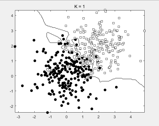
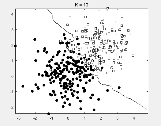
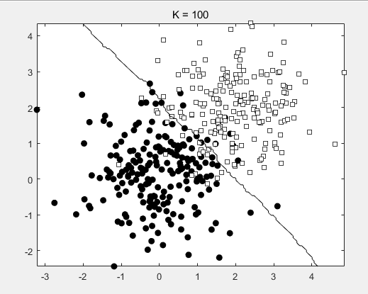
How can you choose a proper K when
dealing with real-world data ?
By validation.
Finish hack.m

function digits = hack(img_name)
%HACK Recognize a CAPTCHA image
%   Inputs:
%       img_name: filename of image
%   Outputs:
%       digits: 1x5 matrix, 5 digits in the input CAPTCHA image.

hack_data = load('hack_data');
% YOUR CODE HERE
X_train = hack_data.X;
y_train = hack_data.y;
X = extract_image(img_name);
K = 10;
digits = knn(X, X_train, y_train, K);

end

the answer of test example I took is :
6|1|5|0|0
-|

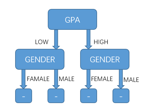
##Decision Tree and ID3

##K-Means Clustering
Implement
k-means algorithm (in kmeans.m)

function [idx, ctrs, iter_ctrs] = kmeans(X, K)
%KMEANS K-Means clustering algorithm
%
%   Input: X - data point features, n-by-p maxtirx.
%          K - the number of clusters
%
%   OUTPUT: idx  - cluster label
%           ctrs - cluster centers, K-by-p matrix.
%           iter_ctrs - cluster centers of each iteration, K-by-p-by-iter
%                       3D matrix.

% YOUR CODE HERE
[N,P] = size(X);
max_iter = 1000;
idx = zeros(1,N);
last_idx = zeros(1,N);
ctrs = reshape(X(unidrnd(N,1,K),:), K, P);
iter_ctrs = zeros(K,P,max_iter);
for iter = 1 : max_iter
    D = pdist2(X, ctrs);
    [~, min_idx] = min(D, [], 2);
    idx = min_idx';
    if idx == last_idx
        break;
    end
    for k = 1 : K
        ctrs(k, :) = mean(X(idx == k, :));
    end
    iter_ctrs(:,:,iter) = ctrs;
    last_idx = idx;
end
iter_ctrs = iter_ctrs(:,:,1:(iter-1));

end

(a) Run your k-means algorithm on kmeans data.mat with the number of clusters K set to 2. Repeat the experiment 1000 times. Use kmeans plot.m to visualize the process of k-means algorithm for the two trials with largest and smallest SD (sum of distances from each point to its respective centroid).

%% Part1
kmeans_data = load('kmeans_data.mat');
X = kmeans_data.X;
K = 2;
[idx, ctrs, iter_ctrs] = kmeans(X, K);
kmeans_plot(X, idx, ctrs, iter_ctrs);

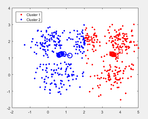
(b) How can we get a stable result using k-means?
By random select several times.
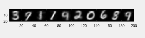
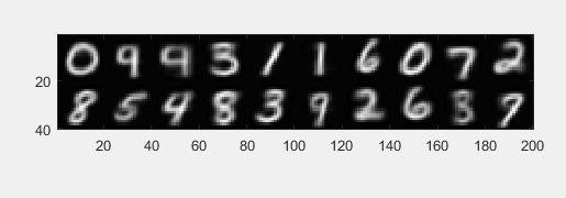
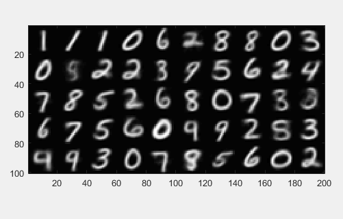
© Run your k-means algorithm on the digit dataset digit data.mat with the number of clusters K set to 10, 20 and 50. Visualize the centroids using show digit.m.

digit_data = load('digit_data.mat');
X = digit_data.X;
K = 10;
% K = 20;
% K = 50;
[idx, ctrs, iter_ctrs] = kmeans(X, K);
show_digit(ctrs);

k=10

k=20

k=50

(d)
Finish vq.m

img = imread('sample1.jpg');
fea = double(reshape(img, size(img, 1)*size(img, 2), 3));
% YOUR (TWO LINE) CODE HERE
[idx, ctrs, iter_ctrs] = kmeans(fea, 64);
fea = ctrs(idx,:);

imshow(uint8(reshape(fea, size(img))));

k=8

k=16

k=32

k=64

origin