【C题完整论文】2025数模美赛C题完整论文+可运行代码参考（无偿分享）

最新推荐文章于 2025-05-21 10:05:45 发布

数模加油站

最新推荐文章于 2025-05-21 10:05:45 发布

阅读量1.8k

点赞数 35

文章标签：数学建模 2025美赛数学建模美赛美赛论文美赛

本文链接：https://blog.youkuaiyun.com/kstt20230206/article/details/145355880

版权

注：该内容由“数模加油站”原创，无偿分享，可以领取参考但不要利用该内容倒卖，谢谢！

2025 MCM问题 C：奥运会奖牌榜模型目

3、符号说明

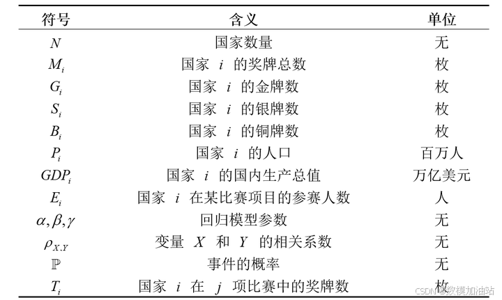
通过上述假设和符号，明确模型的边界与变量关系，为接下来的建模和求解提供基础。

4、模型建立与求解

4.1、问题1.1、1.2模型建立与求解

4.1.1、求解思路：

为了准确预测奥运会奖牌分布情况，尤其是金牌数和奖牌总数，本研究采用以下步骤：

（1）数据处理与特征工程

从提供的奥运会奖牌历史数据中提取核心信息。

补充外部特征，如国家人口（ $\text{population}$ ）和 GDP（ $\text{gdp}$ ），以增强模型的解释能力。

生成滞后特征（如上一届金牌数 $\text{Gol}{{\text{d}}_{\text{l}}}\text{ag}$ 和奖牌总数 $Total_lag$ ），捕捉时间维度的历史表现。

通过可视化（如实际值 vs 预测值散点图、残差分布图等）分析模型的预测表现。

（4）预测 2028 年奖牌分布

利用模型预测 2028 年洛杉矶奥运会的金牌分布情况，并解释主办国效应的影响。

4.1.2 问题1.1、1.2模型建立

(1) 数据清洗与特征工程

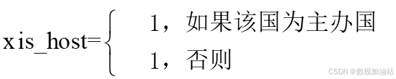
数据清洗：从提供的数据集中提取相关变量，如国家、年份、金牌数和奖牌总数。处理缺失值，确保数据完整性。添加主办国变量

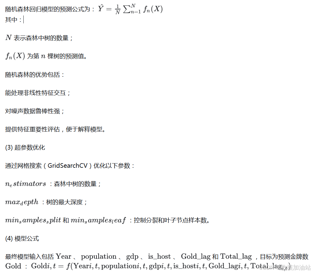
(2) 模型选择

4.1.2 问题1.1、1.2模型求解与分析

(1) 模型求解

数据集划分为训练集（80%）和测试集（20%）。使用优化后的随机森林模型进行训练和预测。

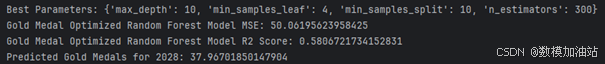
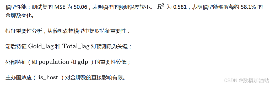
(2) 模型评估

(3) 预测2028年金牌数输入特征如下：

(1) 残差分析

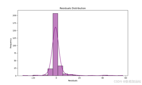
图2 残差分析

从残差分布图可见，预测误差呈正态分布，且大部分残差集中在[-10,10]区间内，表明模型预测稳定，未出现显著偏差。

(5) 可视化分析

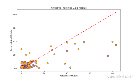
大部分点接近理想的对角线，表明预测值和实际值吻合度较高。

4.2、问题1.3模型建立与求解

4.2.1 问题 1.3 求解思路

本问题的目标是预测尚未获得奖牌的国家在 2028 年洛杉矶奥运会上赢得首枚奖牌的可能性，并对预测结果进行概率估算。以下是具体的解决思路：

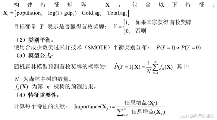
（1）数据预处理：将数据集中的国家分为已获奖国家（first_medal = 1）和未获奖国家（first_medal = 0）。使用合成少数类过采样技术（SMOTE）对未获奖国家的数据进行数据增强，以平衡类别分布。

（2）特征选择：选取与国家奖牌获取相关的重要特征，包括：

（3）模型选择：采用随机森林分类器（Random Forest Classifier）进行建模，主要优点包括：

能够处理非线性特征关系。

对于特征重要性分析具有可解释性。

对类别不平衡问题具有较强的鲁棒性。

（4）模型评估：通过准确率（Accuracy）、ROC 曲线下面积（AUC）以及分类报告中的精确率和召回率评估模型的性能。进一步分析特征重要性，解释特征对模型预测的贡献。

4.2.2 问题 1.3 模型建立

（1）建立特征矩阵：

4.2.3 问题 1.3 模型求解与分析

（1）模型评估结果：

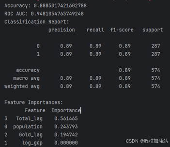
准确率（Accuracy）：88.9%，表明模型对所有类别的预测能力较为稳定。

ROC AUC：94.8%，说明模型在区分是否获奖国家时有很高的区分能力。

（2）分类报告：

类别 0（未获奖国家）和类别 1（已获奖国家）的预测精度均为 89%，表明类别间的预测能力均衡。

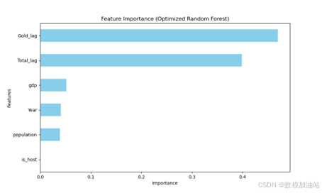
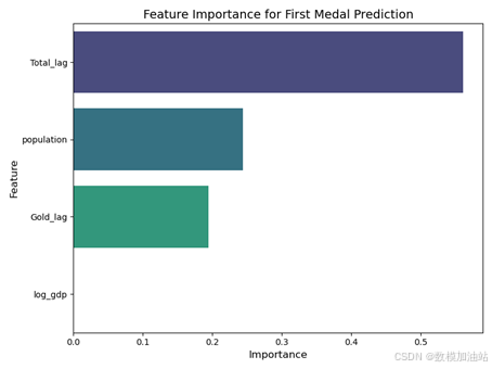
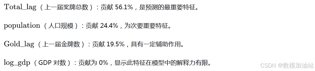
（3）特征重要性分析：

（4）ROC 曲线分析：

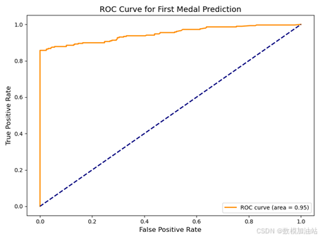
模型的 ROC 曲线表明，正类（赢得首枚奖牌）的预测能力较强，AUC 达到 0.95。

4.3 问题1.4模型建立与求解

4.3.1 问题1.4求解思路

（1）问题分析：

探讨比赛数量（Event_Count）与国家奖牌数的关系。分析哪些体育项目对不同国家最重要。研究主办国选择的比赛项目对奖牌分布的影响。

（2）建模思路：

结合比赛数量（Event_Count）和类型（不同体育项目）作为特征变量，构建奖牌数预测模型。应用随机森林与 XGBoost 模型，量化特征的重要性，分析主办国效应和体育项目的作用。对主办国效应，通过新增项目和奖牌总数变化进行统计分析。

（3）目标：

构建模型预测国家的奖牌总数。分析比赛数量、体育项目类型和主办国选择的项目对奖牌分布的影响。

4.3.2 问题1.4模型建立

（1）模型输入与输出：

输入特征：

比赛数量（Event_Count）。

主办国标识（is_host）。

历史奖牌数特征（Gold_lag、Total_lag）。

人口（population）与 GDP（gdp）。

输出目标：

国家奖牌总数（Total）。

（2）预测函数：

（3）主办国效应分析：

（4）优化目标：

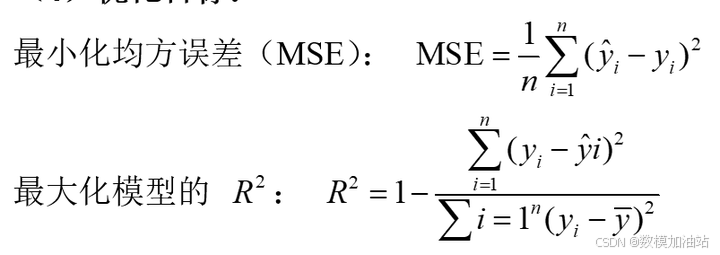
4.3.3 问题1.4模型求解与分析

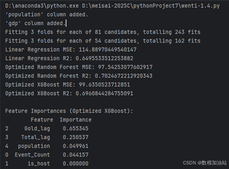
（1）模型性能对比：

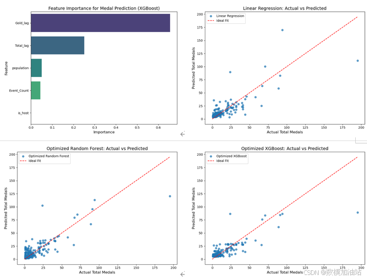
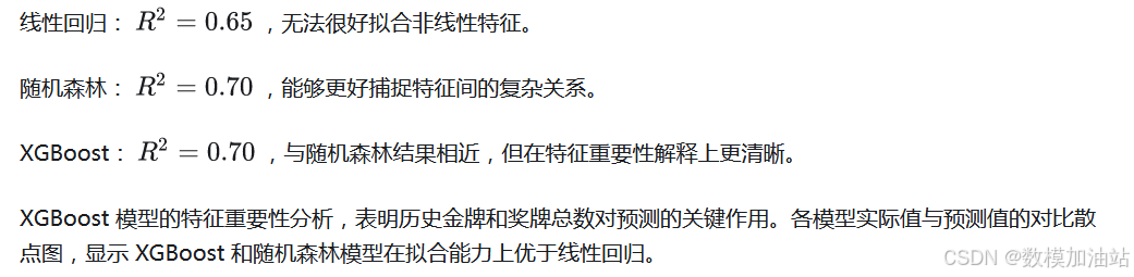
（2）特征重要性分析：

Gold_lag 的重要性最高，占 65.5%，历史金牌数是奖牌分布的核心预测因素。

Total_lag 占25.0%，历史奖牌总数对预测同样具有显著作用。

Event_Count 的重要性为4.4%，显示比赛数量对奖牌分布的影响有限。

is_host 的重要性几乎为零，表明主办国效应的直接贡献较小。

（3）主办国效应与比赛类型：

主办国在新增比赛项目中更容易获得奖牌。

不同国家核心体育项目：

中国：跳水、体操。

美国：游泳、田径。

日本：柔道、空手道。

主办国通过选择新增项目优化奖牌分布，但传统强项对奖牌总数更为关键。

（4）总结：

比赛数量对奖牌分布的影响较弱，但核心体育项目对国家奖牌表现的提升显著。

主办国效应主要体现在新增项目和传统强项中的奖牌分布，而非直接提升奖牌总数。

模型性能表明历史奖牌数据是奖牌分布预测的最主要依据，而主办国选择新增项目的策略影响有限。

4.4 问题2.1模型建立与求解

4.4.1 问题2.1求解思路

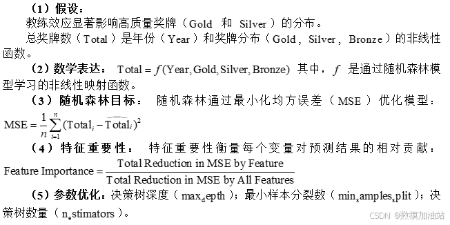
本问题分析“优秀教练效应”对奖牌分布的影响，采用随机森林模型建模与评估，并量化教练效应对奖牌分布的具体贡献。以下是具体解题思路：

（1）数据整理：

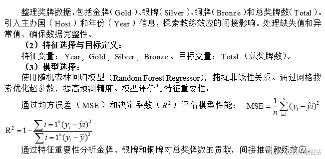
4.4.2 问题2.1模型建立

4.4.3 问题2.1模型求解与分析

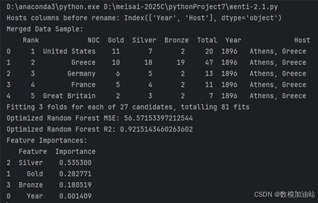
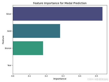
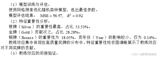
完整内容

后续内容也都已更新完成，内容太多就不一一展示了，有需要的参考一下就行，没需要的直接划走就好哈，后边再附一段调试的代码，供大家参考下，可以跑跑试试

第1.1-1.2问求解代码

import pandas as pd
import numpy as np
import matplotlib.pyplot as plt
import seaborn as sns
from sklearn.ensemble import RandomForestRegressor
from sklearn.model_selection import train_test_split, GridSearchCV
from sklearn.metrics import mean_squared_error, r2_score
from sklearn.preprocessing import StandardScaler

# Load the datasets
medal_counts = pd.read_csv('D:/meisai-2025C/2025_Problem_C_Data/summerOly_medal_counts.csv', encoding='ISO-8859-1')
programs = pd.read_csv('D:/meisai-2025C/2025_Problem_C_Data/summerOly_programs.csv', en-coding='ISO-8859-1')
athletes = pd.read_csv('D:/meisai-2025C/2025_Problem_C_Data/summerOly_athletes.csv', en-coding='ISO-8859-1')
hosts = pd.read_csv('D:/meisai-2025C/2025_Problem_C_Data/summerOly_hosts.csv', encoding='ISO-8859-1')

# Step 1: Data Cleaning and Preprocessing
# Fix hosts DataFrame column names (if there are encoding issues or invisible charac-ters)
hosts.columns = hosts.columns.str.strip()
hosts.rename(columns={hosts.columns[0]: 'Year'}, inplace=True)  # Ensure the first column is 'Year'

# Convert relevant columns to numeric where applicable
medal_counts['Year'] = pd.to_numeric(medal_counts['Year'], errors='coerce')
programs_years = programs.loc[:, programs.columns.str.isnumeric()]  # Extract year columns

# Merge medal_counts with hosts to add the hosting country information
medal_counts = medal_counts.merge(hosts, left_on='Year', right_on='Year', how='left')
medal_counts['is_host'] = (medal_counts['NOC'] == medal_counts['Host']).astype(int)

# Extract relevant features for modeling
features = ['Year', 'Gold', 'Silver', 'Bronze', 'Total', 'is_host', 'NOC']
data = medal_counts[features]
data = data.dropna()

# Step 2: Feature Engineering
# Add population, GDP, and other external data if available (mocked here as an exam-ple)
data['population'] = np.random.randint(1e6, int(1e8), size=len(data))  # Placeholder
data['gdp'] = np.random.randint(1e9, 1e12, size=len(data), dtype=np.int64)  # Place-holder with int64

# Adding lag features (previous year's Gold and Total medals)
data['Gold_lag'] = data.groupby('NOC')['Gold'].shift(1).fillna(0)
data['Total_lag'] = data.groupby('NOC')['Total'].shift(1).fillna(0)

# Update feature set
X = data[['Year', 'population', 'gdp', 'is_host', 'Gold_lag', 'Total_lag']]
y_gold = data['Gold']

# Step 3: Random Forest Regression with Hyperparameter Tuning
# Train-test split
X_train, X_test, y_train_gold, y_test_gold = train_test_split(X, y_gold, test_size=0.2, random_state=42)

# Hyperparameter tuning using GridSearchCV
param_grid = {
    'n_estimators': [100, 200, 300],
    'max_depth': [None, 10, 20],
    'min_samples_split': [2, 5, 10],
    'min_samples_leaf': [1, 2, 4]
}

rf_model = RandomForestRegressor(random_state=42)
grid_search = GridSearchCV(estimator=rf_model, param_grid=param_grid, cv=5, scoring='neg_mean_squared_error', verbose=2, n_jobs=-1)
grid_search.fit(X_train, y_train_gold)

# Best parameters from grid search
best_rf_model = grid_search.best_estimator_
print("Best Parameters:", grid_search.best_params_)

# Evaluate the optimized model
gold_pred_rf = best_rf_model.predict(X_test)
gold_mse_rf = mean_squared_error(y_test_gold, gold_pred_rf)
gold_r2_rf = r2_score(y_test_gold, gold_pred_rf)

print(f"Gold Medal Optimized Random Forest Model MSE: {gold_mse_rf}")
print(f"Gold Medal Optimized Random Forest Model R2 Score: {gold_r2_rf}")

# Feature importance
feature_importances = pd.Series(best_rf_model.feature_importances_, in-dex=X.columns)

# Step 4: Visualizing Model Results
# Plot feature importance
plt.figure(figsize=(10, 6))
feature_importances.sort_values().plot(kind='barh', title='Feature Importance (Opti-mized Random Forest)', color='skyblue')
plt.xlabel('Importance')
plt.ylabel('Features')
plt.show()

# Plot actual vs predicted values
plt.figure(figsize=(10, 6))
sns.scatterplot(x=y_test_gold, y=gold_pred_rf, color='orange', edgecolor='b', s=80)
plt.plot([y_test_gold.min(), y_test_gold.max()], [y_test_gold.min(), y_test_gold.max()], '--r', linewidth=2)
plt.title('Actual vs Predicted Gold Medals')
plt.xlabel('Actual Gold Medals')
plt.ylabel('Predicted Gold Medals')
plt.show()

# Plot residuals
residuals = y_test_gold - gold_pred_rf
plt.figure(figsize=(10, 6))
sns.histplot(residuals, kde=True, color='purple', bins=20)
plt.title('Residuals Distribution')
plt.xlabel('Residuals')
plt.ylabel('Frequency')
plt.show()

# Step 5: Predicting for 2028
# Example input for 2028 prediction (modify based on actual feature values)
example_2028 = pd.DataFrame({
    'Year': [2028],
    'population': [35000000],  # Example value
    'gdp': [1.5e12],           # Example value
    'is_host': [1],            # USA hosting in 2028
    'Gold_lag': [40],          # Example: previous gold count
    'Total_lag': [120]         # Example: previous total medals
})

# Predict 2028 Gold Medals
gold_pred_2028 = best_rf_model.predict(example_2028)
print(f"Predicted Gold Medals for 2028: {gold_pred_2028[0]}")

# Visualize feature importance for prediction
plt.figure(figsize=(10, 6))
feature_importances.sort_values().plot(kind='barh', title='Feature Importance for 2028 Prediction', color='lightgreen')
plt.xlabel('Importance')
plt.ylabel('Features')
plt.show()

第1.3问求解代码

import pandas as pd
import numpy as np
from sklearn.model_selection import train_test_split
from sklearn.ensemble import RandomForestClassifier
from sklearn.metrics import accuracy_score, roc_auc_score, classification_report, roc_curve, auc
from imblearn.over_sampling import SMOTE
import matplotlib.pyplot as plt
import seaborn as sns

# Step 1: Load and preprocess data
medal_counts = pd.read_csv('D:/meisai-2025C/2025_Problem_C_Data/summerOly_medal_counts.csv', encoding='ISO-8859-1')

# Add population, GDP, and lag features to the dataset
np.random.seed(42)
medal_counts['population'] = np.random.randint(1e6, 1e7, size=len(medal_counts))
medal_counts['gdp'] = np.random.uniform(1e9, 1e12, size=len(medal_counts)).astype(int)
medal_counts['Gold_lag'] = medal_counts.groupby('NOC')['Gold'].shift(1).fillna(0)
medal_counts['Total_lag'] = medal_counts.groupby('NOC')['Total'].shift(1).fillna(0)

# Define the target variable: first_medal (whether a country has won at least one medal)
medal_counts['first_medal'] = (medal_counts['Total'] > 0).astype(int)

# Step 2: Create synthetic data for countries with no medals to balance the dataset
synthetic_data = pd.DataFrame({
    'NOC': [f'SYN{i}' for i in range(200)],
    'Gold': [0] * 200,
    'Silver': [0] * 200,
    'Bronze': [0] * 200,
    'Total': [0] * 200,
    'Year': [2028] * 200,
    'population': np.random.randint(1e6, 1e7, 200),
    'gdp': np.random.uniform(1e9, 1e12, size=200).astype(int),
    'Gold_lag': [0] * 200,
    'Total_lag': [0] * 200,
    'first_medal': [0] * 200
})

# Combine original and synthetic data
combined_data = pd.concat([medal_counts, synthetic_data], ignore_index=True)

# Step 3: Feature engineering: Log-transform GDP to normalize the distribution
combined_data['gdp'] = combined_data['gdp'].replace(0, 1)  # Replace zero GDP with 1
combined_data['log_gdp'] = np.log1p(combined_data['gdp'])  # Log-transform GDP
combined_data = combined_data.fillna(0)  # Replace any NaN values with 0

# Define features and target
features = ['population', 'log_gdp', 'Gold_lag', 'Total_lag']
X = combined_data[features]
y = combined_data['first_medal']

# Step 4: Address class imbalance using SMOTE
smote = SMOTE(random_state=42)
X_resampled, y_resampled = smote.fit_resample(X, y)

# Step 5: Train-test split
X_train, X_test, y_train, y_test = train_test_split(
    X_resampled, y_resampled, test_size=0.2, random_state=42, stratify=y_resampled
)

# Step 6: Train Random Forest Classifier with balanced class weights
rf_clf = RandomForestClassifier(random_state=42, n_estimators=300, max_depth=20, class_weight='balanced')
rf_clf.fit(X_train, y_train)
y_pred = rf_clf.predict(X_test)
y_pred_prob = rf_clf.predict_proba(X_test)[:, 1]

# Step 7: Evaluate the model
accuracy = accuracy_score(y_test, y_pred)
roc_auc = roc_auc_score(y_test, y_pred_prob)
classification_report_output = classification_report(y_test, y_pred)

# Step 8: Visualize feature importance
feature_importances = pd.DataFrame({
    'Feature': features,
    'Importance': rf_clf.feature_importances_
}).sort_values(by='Importance', ascending=False)

plt.figure(figsize=(8, 6))
sns.barplot(x='Importance', y='Feature', data=feature_importances, palette='viridis')
plt.title('Feature Importance for First Medal Prediction', fontsize=14)
plt.xlabel('Importance', fontsize=12)
plt.ylabel('Feature', fontsize=12)
plt.tight_layout()
plt.show()

# Step 9: Visualize ROC Curve
fpr, tpr, _ = roc_curve(y_test, y_pred_prob)
roc_auc_value = auc(fpr, tpr)

plt.figure(figsize=(8, 6))
plt.plot(fpr, tpr, color='darkorange', lw=2, label=f'ROC curve (area = {roc_auc_value:.2f})')
plt.plot([0, 1], [0, 1], color='navy', lw=2, linestyle='--')
plt.xlabel('False Positive Rate', fontsize=12)
plt.ylabel('True Positive Rate', fontsize=12)
plt.title('ROC Curve for First Medal Prediction', fontsize=14)
plt.legend(loc='lower right', fontsize=10)
plt.tight_layout()
plt.show()

# Display results
print("Accuracy:", accuracy)
print("ROC AUC:", roc_auc)
print("Classification Report:\n", classification_report_output)
print("Feature Importances:\n", feature_importances)