


大家好,我是小白鸽,本期为大家分享如何用GeoPandas进行空间数据分析。文章首先对GeoPandas进行了简要介绍,其次对GeoPandas的数据结构做了介绍,然后就GeoPandas的主要功能使用展示了代码示例,最后结合案例对GeoPandas功能做了补充介绍。
GeoPandas简介
GeoPandas 是一个开源的Python 库,用于处理和分析地理空间数据。它建立在 Pandas 库之上,并添加了对几何形状和空间操作的支持。这使得 GeoPandas 成为处理地理空间数据的重要工具。
GeoPandas 主要功能
-
地理数据类型: GeoPandas 支持多种几何数据类型,包括点、线、多边形和几何集合。
-
空间操作: GeoPandas 提供了丰富的空间操作函数,例如缓冲区生成、裁剪、合并、分割、拓扑运算等。
-
地图绘制: GeoPandas 可以与matplotlib 等绘图库集成,轻松创建地图和空间数据可视化。
-
数据分析: GeoPandas 可以进行各种空间数据分析,例如计算几何图形的面积、长度、质心等属性,以及进行空间统计分析。
-
数据导入和导出: GeoPandas 支持多种地理数据格式,例如 Shapefile、GeoJSON、GML、KML 等,方便进行数据交换和共享。
GeoPandas数据结构
-
GeoSeries
GeoSeries 是GeoPandas 的基本数据结构,它是一个类似 Pandas 的 Series,但是专门用于存储几何对象。每个元素都是一个几何形状,可以是点、线、多边形等。
主要属性和方法:
geometry: 返回一个包含所有几何对象的列表。
crs: 表示坐标参考系(Coordinate Reference System, CRS)的信息。
area: 计算每个几何对象的面积。
boundary: 返回每个几何对象的边界。
centroid: 返回每个几何对象的重心(质心)。
contains: 判断几何对象是否包含另一个几何对象。
distance: 计算两个几何对象之间的最短距离。
intersection: 计算两个几何对象的交集。
buffer: 为几何对象生成缓冲区。
创建 GeoSeries 示例:
import geopandas as gpd
from shapely.geometry import Point
# 创建一个包含点的GeoSeries
points = gpd.GeoSeries([Point(1, 1), Point(2, 2), Point(3, 3)])
print(points)
GeoDataFrame-
GeoDataFrame
GeoDataFrame 是GeoPandas 的另一个核心数据结构,它是 DataFrame 的扩展,专门用于处理包含几何数据的表格数据。GeoDataFrame 有一个特殊的列,通常命名为 geometry,用于存储几何对象。
主要属性和方法:
geometry: 特殊的列,用于存储几何数据。
crs: 表示整个GeoDataFrame 的坐标参考系。
to_crs: 将GeoDataFrame 的坐标参考系转换为新系统。
plot: 绘制GeoDataFrame 中的几何对象。
geom_type: 返回几何类型。
buffer: 为GeoDataFrame 中的所有几何对象生成缓冲区。
centroid: 返回GeoDataFrame 中所有几何对象的重心。
创建 GeoDataFrame 示例:
import geopandas as gpd
from shapely.geometry import Polygon
# 创建一个多边形
polygon = Polygon([(0, 0), (1, 0), (1, 1), (0, 1)])
# 创建一个 GeoDataFrame
gdf = gpd.GeoDataFrame({'geometry': [polygon]})
print(gdf)
功能示例
-
矢量数据读写
import geopandas as gpd from shapely.geometry import Point # 生成虚拟POI数据(咖啡店) poi_data = { 'name': ['Starbucks', 'Luckin Coffee', 'Costa'], 'geometry': [Point(116.3, 39.9), Point(116.31, 39.91), Point(116.29, 39.88)] } poi_gdf = gpd.GeoDataFrame(poi_data, crs="EPSG:4326") # WGS84坐标系 # 生成虚拟地铁站数据 metro_data = { 'station': ['Station_A', 'Station_B'], 'geometry': [Point(116.305, 39.905), Point(116.31, 39.895)] } metro_gdf = gpd.GeoDataFrame(metro_data, crs="EPSG:4326") # 保存为Shapefile和GeoJSON poi_gdf.to_file("poi_data.shp") # 写入Shapefile metro_gdf.to_file("metro_data.geojson", driver='GeoJSON') # 写入GeoJSON # 从文件读取数据 poi = gpd.read_file("poi_data.shp") metro = gpd.read_file("metro_data.geojson") -
空间连接
# 创建地铁站500米缓冲区(转换为投影坐标系计算距离) metro_projected = metro.to_crs(epsg=32650) # UTM 50N metro_projected['buffer'] = metro_projected.geometry.buffer(500) # 500米缓冲区 # 将POI数据也转换到同一坐标系 poi_projected = poi.to_crs(metro_projected.crs) # 空间连接:找出位于缓冲区内的POI joined = gpd.sjoin( poi_projected, metro_projected[['station', 'buffer']].set_geometry('buffer'), how='inner', predicate='within' ) print("地铁站500米范围内的POI:") print(joined[['name', 'station']]) -
缓冲区分析
import matplotlib.pyplot as plt
# 创建可视化画布
fig, ax = plt.subplots(figsize=(10, 8))
# 绘制原始地铁站
metro.plot(ax=ax, color='red', markersize=100, label='Metro Stations')
# 绘制缓冲区
metro_projected.set_geometry('buffer').plot(
    ax=ax,
    alpha=0.3,
    edgecolor='blue',
    facecolor='none',
    label='500m Buffer'
)
# 绘制POI点
poi.plot(ax=ax, color='green', markersize=50, label='POI')
# 添加图例和标题
plt.legend()
plt.title("Metro Station Buffers and POI Distribution")
plt.show()
-
坐标转换
# 查看原始坐标系
print("POI数据坐标系:", poi.crs)  # EPSG:4326 (WGS84)
# 转换为Web墨卡托投影(EPSG:3857)
poi_web_mercator = poi.to_crs(epsg=3857)
print("转换后坐标系:", poi_web_mercator.crs)
# 坐标系转换前后坐标示例
print("\n原始坐标(WGS84):")
print(poi.geometry.head())
print("\n转换后坐标(Web墨卡托):")
print(poi_web_mercator.geometry.head())
案例分享
-
背景
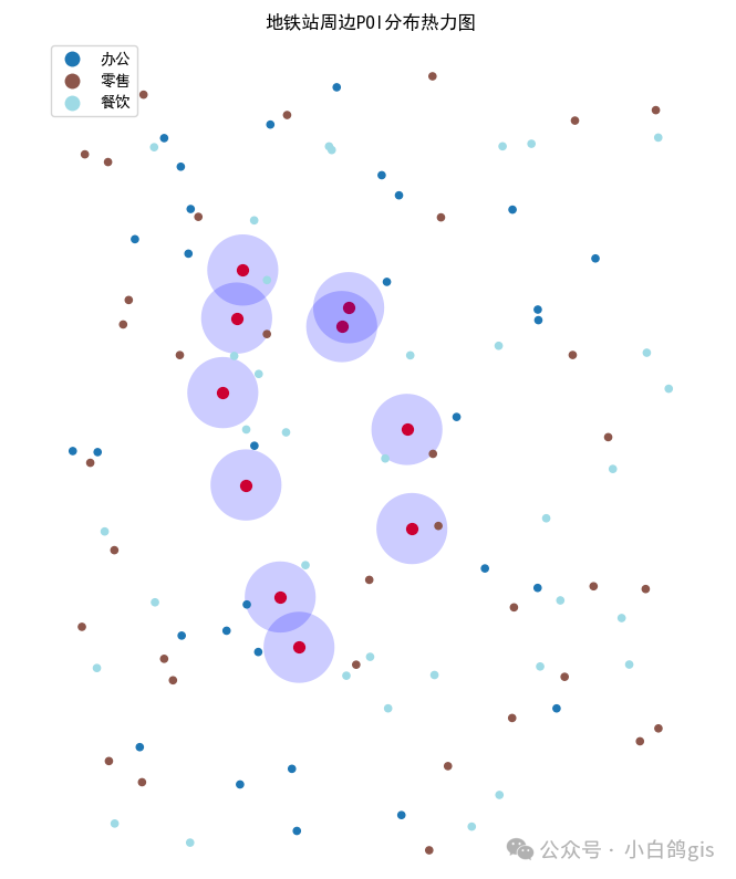
假设现在有地铁站点数据和Poi数据,需要分析地铁站与Poi的关系,并且求出每个地铁站1km范围内的Poi数量。
-
代码示例
import contextily as ctx
import matplotlib.pyplot as plt
import geopandas as gpd
from shapely.geometry import Point
# 生成模拟数据(100个随机POI和10个地铁站)
import numpy as np
np.random.seed(42)
# 生成随机POI(北京范围)
poi_points = [Point(lon, lat) for lon, lat in
             zip(np.random.uniform(116.2, 116.4, 100),
                 np.random.uniform(39.8, 40.0, 100))]
poi_gdf = gpd.GeoDataFrame(
    geometry=poi_points,
    data={'category': np.random.choice(['餐饮', '零售', '办公'], 100)},
    crs="EPSG:4326"
)
# 生成地铁站
metro_points = [Point(lon, lat) for lon, lat in
               zip(np.random.uniform(116.25, 116.35, 10),
                   np.random.uniform(39.85, 39.95, 10))]
metro_gdf = gpd.GeoDataFrame(
    geometry=metro_points,
    data={'station': [f'Station_{i}' for i in range(10)]},
    crs="EPSG:4326"
)
# 分析每个地铁站1km范围内的POI数量
metro_proj = metro_gdf.to_crs(epsg=32650)
metro_proj['buffer'] = metro_proj.geometry.buffer(1000)
poi_proj = poi_gdf.to_crs(metro_proj.crs)
joined = gpd.sjoin(
    poi_proj,
    metro_proj.set_geometry('buffer'),
    how='inner',
    predicate='within'
)
# 统计结果
result = joined.groupby('station').agg(
    total_poi=('category', 'count'),
    restaurant_count=('category', lambda x: (x=='餐饮').sum())
).reset_index()
print("\n各地铁站周边POI统计:")
print(result)
# 可视化
fig, ax = plt.subplots(figsize=(12, 10))
# 绘制底图
metro_proj.to_crs(epsg=3857).plot(
    ax=ax,
    color='red',
    markersize=50,
    label='Metro Stations'
)
metro_proj.set_geometry('buffer').to_crs(epsg=3857).plot(
    ax=ax,
    alpha=0.2,
    color='blue'
)
poi_proj.to_crs(epsg=3857).plot(
    ax=ax,
    column='category',
    legend=True,
    markersize=20,
    categorical=True,
    cmap='tab20'
)
# 添加底图瓦片
#OpenStreetMap的底图不一定能连接上,建议换自己的底图或者删除本行
ctx.add_basemap(ax, source=ctx.providers.OpenStreetMap.Mapnik)
plt.title("地铁站周边POI分布热力图")
plt.axis('off')
plt.show()
-
结果
更多内容
Deepseek与规划协同:填平技术门槛,利用Deepseek进行空间句法分析
更多内容可以关注微信公众号“小白鸽gis”


 75
75

 被折叠的 条评论
为什么被折叠?
被折叠的 条评论
为什么被折叠?
 到【灌水乐园】发言


