【DataWhales】深入浅出Pytorch-第二章

1. Pytorch的基本操作

1.1 建立tensor类型（2种方法）

1. torch.tensor(data,*,dtype=)
int类型默认是int32。

   import torch
   # 创建tensor,用dtype指定类型。注意类型要匹配
   a = torch.tensor(1.0, dtype=torch.float)
   b = torch.tensor(1 , dtype=torch.long)
   c = torch.tensor(1.0 , dtype=torch.int8)
   print(a, b, c)
   

2. torch.FloatTensor；torch.IntTensor；torch.IntTensor

   # 使用指定类型函数随机初始化指定大小的tensor
   d = torch.FloatTensor(2,3)
   e = torch.IntTensor(2)
   f = torch.IntTensor([1, 2, 3, 4])
   print(d,'\n' ,e, '\n', f )
   

1.2 tensor 与 numpy(array)之间的转换

1. array to numpy

   # tensor 和 numpy array 之间的相互转换
   import numpy as np
   g = np.array([[1, 2, 3],[4, 5, 6]])
   h = torch.tensor(g)
   print(h)
   i = torch.from_numpy(g)
   print(i)
   

2. torch to array

   # tensor 和 numpy array 之间的相互转换
   import numpy as np
   g = np.array([[1, 2, 3],[4, 5, 6]])
   h = torch.tensor(g)
   j = h.numpy()
   print(j)
   

   [[1 2 3]
    [4 5 6]]
   

1.3 tensor常见的构造函数（4个函数）

arange是左开右闭。

rand; ones; zeros; arange

# 常见的构造Tensor的函数
k = torch.rand(2,3)
l = torch.ones(2,3)
m = torch.zeros(2,3)
n = torch.arange(0,10,2)
print(k, '\n', l, '\n', m, '\n', n)

tensor([[0.9137, 0.4723, 0.5141],
        [0.0574, 0.3423, 0.1671]]) 
tensor([[1., 1., 1.],
        [1., 1., 1.]]) 
tensor([[0., 0., 0.],
        [0., 0., 0.]]) 
tensor([0, 2, 4, 6, 8])

2. Tensor的基本操作

2.1 查看tensor的维度信息（2种方式）

# 查看tensor的维度信息（两种方式）
print(k.shape)
print(k.size())

2.2 tensor的运算

与矩阵计算类似。

# tensor的运算
o = torch.add(1,k)
print(o)

tensor([[1.9137, 1.4723, 1.5141],
        [1.0574, 1.3423, 1.1671]])

2.3 tensor索引

1. 与numpy类似，用$\text{中括号}$，是$\text{从第0个时开始计数}$。

   # 索引方式，与numpy类似
   print(o[:,1])
   print(o[0,:])
   

   tensor([1.4723, 1.3423])
   tensor([1.9137, 1.4723, 1.5141])
   

2.4 改变形状（view）

1. $\text{固定特定的行与列}$

   print(o.view((3,2)))
   

   tensor([[1.9137, 1.4723],
           [1.5141, 1.0574],
           [1.3423, 1.1671]])
   

2. $\text{只固定行/列}$，另外$\text{不确定的列/行用-1表示}$，torch会$\text{自动计算出对应的列/行}$。

   print(o.view(-1,2))
   

   tensor([[1.9137, 1.4723],
           [1.5141, 1.0574],
           [1.3423, 1.1671]])
   

2.5 扩展&压缩tensor的维度：unsqueeze/squeeze

因为unsqueeze/squeeze $\text{只对维度为1}$的进行操作。

1. 先进性扩展unsqueeze

   print(o)
   r = o.unsqueeze(1)
   print(r)
   print(r.shape)
   

   tensor([[1.2652, 1.0650, 1.5593],
           [1.7864, 1.0015, 1.4458]])
   tensor([[[1.2652, 1.0650, 1.5593]],
   
           [[1.7864, 1.0015, 1.4458]]])
   torch.Size([2, 1, 3])
   

2. 在对tensor进行压缩squeeze。$\text{只对维度为1}$的进行操作。

   s = r.squeeze(0)
   print(s)
   print(s.shape)
   

   tensor([[[1.2652, 1.0650, 1.5593]],
   
           [[1.7864, 1.0015, 1.4458]]])
   torch.Size([2, 1, 3])
   

3. $\text{只对维度为1}$的进行操作。

   t = r.squeeze(1)
   print(t)
   print(t.shape)
   

   tensor([[1.2652, 1.0650, 1.5593],
           [1.7864, 1.0015, 1.4458]])
   torch.Size([2, 3])
   

3. 自动求导

自动求导主要用于反向传播，Tensor数据结构是实现自动求导的基础。

3.1 数学基础

• 多元函数求导的雅克比矩阵
  $$J=\left(\begin{array}{ccc}\frac{\partial y_1}{\partial x_1}& \cdots & \frac{\partial y_1}{\partial x_n}\\ ⋮& \ddots & ⋮\\ \frac{\partial y_m}{\partial x_1}& \cdots & \frac{\partial y_m}{\partial x_n}\end{array}\right)\text{\hspace{1em}(1)}$$
• 复合函数求导的链式法则 若$h(x)=f(g(x))$，则$h^{\prime }(x)=f^{\prime }(g(x))\cdot g^{\prime }(x)$。
• 假设是一层神经网络，则$\text{PyTorch自动求导提供了计算雅克比乘积的工具}$。
  • 损失函数$l$对输出$y$的导数是：
    $$v=\left(\begin{array}{lll}\frac{\partial l}{\partial y_1}& \cdots & \frac{\partial l}{\partial y_m}\end{array}\right)\text{\hspace{1em}(2)}$$
  • 那么$l$对输入$x$的导数就是 :
    $$vJ=\left(\begin{array}{ccc}\frac{\partial l}{\partial y_1}& \cdots & \frac{\partial l}{\partial y_m}\end{array}\right)\left(\begin{array}{ccc}\frac{\partial y_1}{\partial x_1}& \cdots & \frac{\partial y_1}{\partial x_n}\\ ⋮& \ddots & ⋮\\ \frac{\partial y_m}{\partial x_1}& \cdots & \frac{\partial y_m}{\partial x_n}\end{array}\right)=\left(\begin{array}{lll}\frac{\partial l}{\partial x_1}& \cdots & \frac{\partial l}{\partial x_n}\end{array}\right)\text{\hspace{1em}(3)}$$

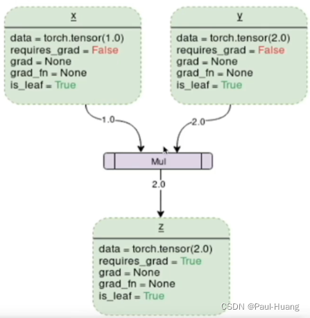
3.2 动态计算图

张量和运算结合起来创建动态计算图

3.3 设置每个变量自动求导

1. 允许每个变量求导

   import torch
   x1 = torch.tensor(1.0, requires_grad=True)
   x2 = torch.tensor(2.0, requires_grad=True)
   y = x1 + 2*x2
   print(y)
   # 首先查看每个变量是否需要求导
   print(x1.requires_grad)
   print(x2.requires_grad)
   print(y.requires_grad)
   

   tensor(5., grad_fn=<AddBackward0>)
   True
   True
   True
   

2. 不允许每个变量求导

   # 尝试，如果不允许求导，会出现什么情况？
   x1 = torch.tensor(1.0, requires_grad=False)
   x2 = torch.tensor(2.0, requires_grad=False)
   y = x1 + 2*x2
   y.backward()
   

   ---------------------------------------------------------------------------
   RuntimeError                              Traceback (most recent call last)
   /tmp/ipykernel_11770/4087792071.py in <module>
         3 x2 = torch.tensor(2.0, requires_grad=False)
         4 y = x1 + 2*x2
   ----> 5 y.backward()
   
   /data1/ljq/anaconda3/envs/smp/lib/python3.8/site-packages/torch/_tensor.py in backward(self, gradient, retain_graph, create_graph, inputs)
       253                 create_graph=create_graph,
       254                 inputs=inputs)
   --> 255         torch.autograd.backward(self, gradient, retain_graph, create_graph, inputs=inputs)
       256 
       257     def register_hook(self, hook):
   
   /data1/ljq/anaconda3/envs/smp/lib/python3.8/site-packages/torch/autograd/__init__.py in backward(tensors, grad_tensors, retain_graph, create_graph, grad_variables, inputs)
       145         retain_graph = create_graph
       146 
   --> 147     Variable._execution_engine.run_backward(
       148         tensors, grad_tensors_, retain_graph, create_graph, inputs,
       149         allow_unreachable=True, accumulate_grad=True)  # allow_unreachable flag
   
   RuntimeError: element 0 of tensors does not require grad and does not have a grad_fn
   

3.4 查看每个变量导数大小

1. 没有反向传播

   # 查看每个变量导数大小。此时因为还没有反向传播，因此导数都不存在
   print(x1.grad.data)
   print(x2.grad.data)
   print(y.grad.data)
   

   AttributeError                            Traceback (most recent call last)
   /tmp/ipykernel_11770/1707027577.py in <module>
         1 # 查看每个变量导数大小。此时因为还没有反向传播，因此导数都不存在
   ----> 2 print(x1.grad.data)
         3 print(x2.grad.data)
         4 print(y.grad.data)
   
   AttributeError: 'NoneType' object has no attribute 'data'
   

2. 反向传播后看大小

   ## 反向传播后看导数大小
   y = x1 + 2*x2
   y.backward()
   print(x1.grad.data)
   print(x2.grad.data)
   

   tensor(1.)
   tensor(2.)
   

3. $\text{导数是会累积的，重复运行相同命令，grad会增加}$（此处运行5次）

   # 导数是会累积的，重复运行相同命令，grad会增加
   y = x1 + 2*x2
   y.backward()
   print(x1.grad.data)
   print(x2.grad.data)
   

   tensor(5.)
   tensor(10.)
   

   所以每次计算前需要清除当前导数值避免累积，这一功能可以通过pytorch的optimizer实现。

4. 并行计算

1. 为什么?
   • 能计算——显存占用-算得快
   • 计算速度
   • 效果好
   • 大batch提升训练效果
2. 怎么并行?———CUDA
   • GPU厂商NVIDIA提供的GPU计算框架
   • GPU本身的编程基于CUDA语言实现
   • 在PyTorch中，CUDA的含义有所不同
   • 更多的指使用GPU进行计算（而不是CPU )
3. 并行的方法
   • 网络结构分布到不同设备中(Network Partitioning)
   • 同一层的任务分布到不同数据中(Layer-wise Partitioning)
   • 不同数据分布到不同的设备中(Data Parallelism)

常见的方法是$\text{不同数据分布到不同的设备中(Data Parallelism)}$。