caffe实战之opencv

原文：https://blog.youkuaiyun.com/hellohaibo/article/details/77761880

Caffe实战Day1-准备训练数据

1、准备数据集

这一步就是想方设法搞来训练数据，可以是图像，可以是语音文件、视频等等。

ok，现在假设你找到了所需的数据集（本教程就以图片为例），数据集需要进行预处理，这部分工作量比较大，需要将庞大的数据集人工分类好。

每个文件夹下就是相应的图片，然后将每一类的图片重命名，切记：不同类的图片要有区别，比如bus类的图片命名为300-399（因为我这里每一类的图片不超过100张，所以用三位数表示，一般命名为六位数数字串），dinosaur类图片为400-499....以此类推，命名完所有类别图片。

2、制作训练集(train)及验证集(val)

第一步当然是新建两个文件夹train和val用来存放训练集、验证集。

第二步确定训练集大小和验证集大小，比如在本教程，我使用了一共五类图片共500张，每种100张，我的选择是每类图片中20张用于验证，80张用于训练，即train文件夹里面共有400张图片，val文件夹下共有100张图片。

下图是train文件夹下的图片：

下图时val文件夹下的图片：

如图所示我是把每类中的*00-*19号丢进val文件夹里面，*20-*99丢进train文件夹里。

第三步整理图片

这一步实现方法很多，C++/Python/sh脚本等等，我们这里使用python，原因是代码简洁且简单。

不过要先新建两个txt文件train.txt和val.txt用来保存图片名称和对应标签。

get_data.py

[python] view plain copy

1. # -*- coding: UTF-8 -*-  
2.   
3. # Author:dasuda  
4. # Date:2017.8.18  
5.   
6. import os  
7. import re  
8.   
9. path_train = "train文件夹路径" #建议是用绝对路径  
10. path_val = "val文件夹路径"  
11.   
12. if not os.path.exists(path_train):  
13.     print "path_train not exist!!!"  
14.     ox._exit()  
15. else:  
16.     print "path_train exist!!!"  
17.   
18. if not os.path.exists(path_val):  
19.     print "path_val not exist!!!"  
20.     ox._exit()  
21. else:  
22.     print "path_val exist!!!"  
23.   
24. file_train = open('train.txt的路径','wt')  
25. file_val = open('val.txt的路径','wt')  
26.   
27. file_train.truncate()  
28. file_val.truncate()  
29.   
30. pa = r".+(?=\.)"  
31. pattern = re.compile(pa)  
32.   
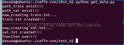
33. print "now,creating train.txt..."  
34. for filename in os.listdir(path_train):  
35. #   print filename  
36. #   abspath = os.path.join(path_train,filename);  
37.     group_lable = pattern.search(filename)  
38.     str_label = str(group_lable.group())  
39.     if str_label[0]=='3':  
40.         train_lable = '0'  
41.     elif str_label[0]=='4':  
42.         train_lable = '1'  
43.     elif str_label[0]=='5':  
44.         train_lable = '2'  
45.     elif str_label[0]=='6':  
46.         train_lable = '3'  
47.     elif str_label[0]=='7':  
48.         train_lable = '4'  
49.     else:  
50.         print "error data!!!"  
51.         ox._exit()  
52. #   print abspath,train_lable.group()  
53.     file_train.write(filename+' '+train_lable+'\n')  
54. print "train.txt created!!!"  
55. print "-----------------------------------"  
56. print "now,creating val.txt..."  
57. for filename in os.listdir(path_val):  
58. #   print filename  
59. #   abspath = os.path.join(path_val,filename);  
60.     group_lable = pattern.search(filename)  
61.     str_label = str(group_lable.group())  
62.     if str_label[0]=='3':  
63.         val_lable = '0'  
64.     elif str_label[0]=='4':  
65.         val_lable = '1'  
66.     elif str_label[0]=='5':  
67.         val_lable = '2'  
68.     elif str_label[0]=='6':  
69.         val_lable = '3'  
70.     elif str_label[0]=='7':  
71.         val_lable = '4'  
72.     else:  
73.         print "error data!!!"  
74.         ox._exit()  
75. #   print abspath,train_lable.group()  
76.     file_val.write(filename+' '+val_lable+'\n')  
77. print "val.txt created!!!"  
78.   
79. print "function over!!!"  

执行完之后，若路径都正确，命令行输出为：

接下来查看一下train.txt和val.txt的内容(乱序排列)

下面附上我的代码

# -*- coding: UTF-8 -*-  
      
import os  
import re  
      
path_train = "/home/hp/caffe/mytest1/re/train/" #建议是用绝对路径  
path_val = "/home/hp/caffe/mytest1/re/test/"  
      
if not os.path.exists(path_train):  
        print "path_train not exist!!!"  
        ox._exit()  
else:  
        print "path_train exist!!!"  
      
if not os.path.exists(path_val):  
        print "path_val not exist!!!"  
        ox._exit()  
else:  
        print "path_val exist!!!"  
      
file_train = open('/home/hp/caffe/mytest1/zhn/train.txt','wt')  
file_val = open('/home/hp/caffe/mytest1/zhn/val.txt','wt')  
      
file_train.truncate()  
file_val.truncate()  
      
pa = r".+(?=\.)"  
pattern = re.compile(pa)  
      
print "now,creating train.txt..."  
for filename in os.listdir(path_train):  
#   print filename  
#abspath = os.path.join(path_train,filename);  
        group_lable = pattern.search(filename)  
        str_label = str(group_lable.group())  
        if str_label[0]=='3':  
           train_lable = '0'  
        elif str_label[0]=='4':  
           train_lable = '1'  
        elif str_label[0]=='5':  
           train_lable = '2'  
        elif str_label[0]=='6':  
           train_lable = '3'  
        elif str_label[0]=='7':  
           train_lable = '4'  
        else:  
           print "error data!!!"  
           ox._exit()  
#   print abspath,train_lable.group()  
        file_train.write(filename+' '+train_lable+'\n')  
print "train.txt created!!!"  
print "-----------------------------------"  
print "now,creating val.txt..."  
for filename in os.listdir(path_val):  
#   print filename  
#abspath = os.path.join(path_val,filename);  
        group_lable = pattern.search(filename)  
        str_label = str(group_lable.group())  
        if str_label[0]=='3':  
            val_lable = '0'  
        elif str_label[0]=='4':  
            val_lable = '1'  
        elif str_label[0]=='5':  
            val_lable = '2'  
        elif str_label[0]=='6':  
            val_lable = '3'  
        elif str_label[0]=='7':  
            val_lable = '4'  
        else:  
            print "error data!!!"  
            ox._exit()  
    #   print abspath,train_lable.group()  
        file_val.write(filename+' '+val_lable+'\n')  
print "val.txt created!!!"  
      
print "function over!!!"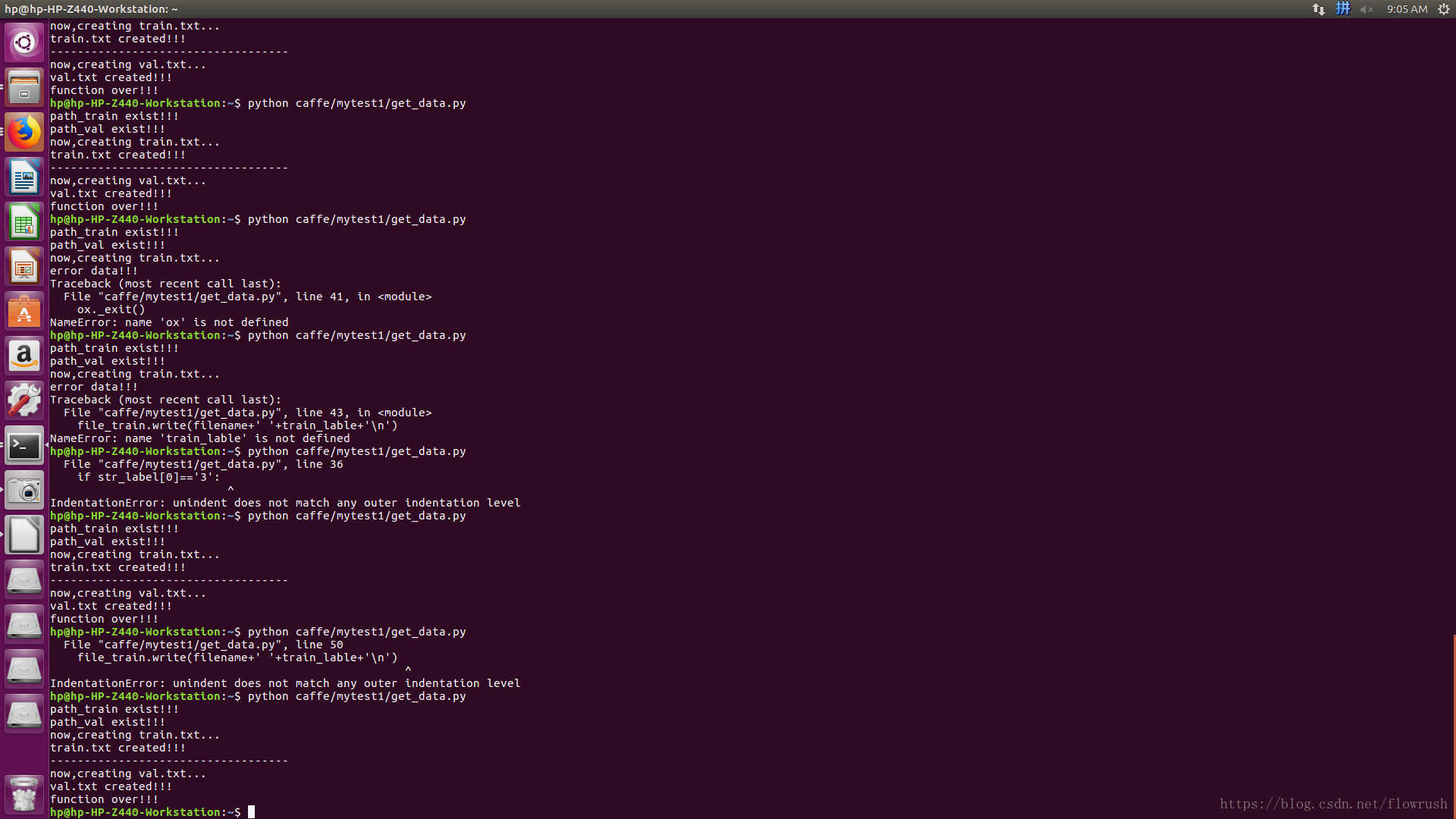  

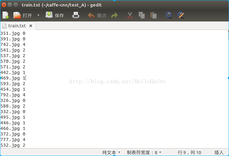
注意缩进，不然报错。

这里提一下：网上各种各样的教程txt文件格式可谓是五花八门，谁也没说清楚，为什么是这样的格式，为什么不是那样的格式，在这里澄清一下，这里的txt格式没有固定的格式，他只是生成lmdb的中间文件，他这里的格式只与生成lmdb时有关，等到下一节讲解怎样生成lmdb文件时候，你就会恍然大悟。我的建议是：txt里面命名尽可能简单，最好是像我这样，直接-文件名 标签。

Caffe实战Day2-准备lmdb文件和均值文件

友情链接：我的caffe实战Day1-准备训练数据

OK，上篇文章我们已经生成两个txt文件，分别是train.txt和val.txt，训练数据和测试数据的标签文件。

一、生成lmdb文件

本次我们要生成能让网络结构文件“读懂”的标签文件格式——lmdb，其实还有很多其它格式：leveldb、hdf5等等。

那么我们是以哪种形式生成lmdb文件呢？用的是caffe提供的convert_imageset功能，让txt格式文件转换成lmdb格式

我们通过以下脚本实现转换：

注意：其中注释的地方，那些地方是你需要根据你的实际情况进行修改的

[php] view plain copy

1. #!/usr/bin/env sh  
2.   
3. EXAMPLE=/home/dasuda/caffe-cnn/test_A #工程的路径   
4. DATA=/home/dasuda/caffe-cnn/test_A #工程的路径   
5. TOOLS=/home/dasuda/caffe/tools #caffe工具路径   
6.   
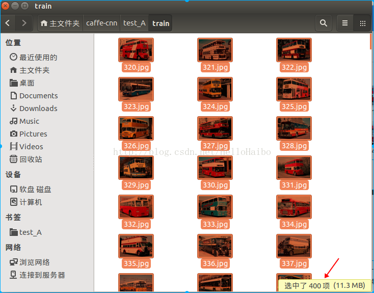
7. TRAIN_DATA_ROOT=/home/dasuda/caffe-cnn/test_A/train/ #训练集路径   
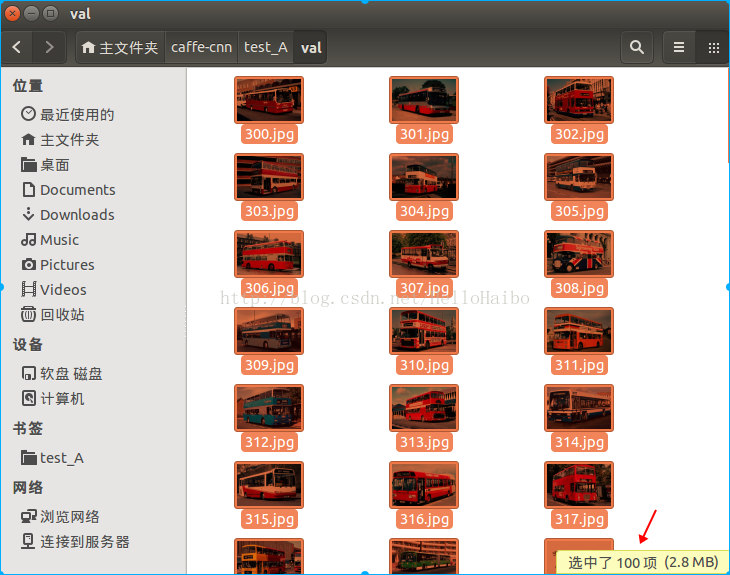
8. VAL_DATA_ROOT=/home/dasuda/caffe-cnn/test_A/val/ #测试集路径   
9.   
10. # Set RESIZE=true to resize the images to 256x256. Leave as false if images have  
11. # already been resized using another tool.  
12. RESIZE=true #这里是resize图片，我这里时开启此功能，resize成256*256  
13. if $RESIZE; then  
14.   RESIZE_HEIGHT=256  
15.   RESIZE_WIDTH=256  
16. else  
17.   RESIZE_HEIGHT=0  
18.   RESIZE_WIDTH=0  
19. fi  
20.   
21. if [ ! -d "$TRAIN_DATA_ROOT" ]; then  
22.   echo "Error: TRAIN_DATA_ROOT is not a path to a directory: $TRAIN_DATA_ROOT"  
23.   echo "Set the TRAIN_DATA_ROOT variable in create_imagenet.sh to the path" \  
24.        "where the ImageNet training data is stored."  
25.   exit 1  
26. fi  
27.   
28. if [ ! -d "$VAL_DATA_ROOT" ]; then  
29.   echo "Error: VAL_DATA_ROOT is not a path to a directory: $VAL_DATA_ROOT"  
30.   echo "Set the VAL_DATA_ROOT variable in create_imagenet.sh to the path" \<strong>  
31. </strong>       "where the ImageNet validation data is stored."  
32.   exit 1  
33. fi  
34.   
35. #训练_lmdb  
36. echo "Creating train lmdb..."  
37.   
38. #生成前需要先删除已有的文件夹 必须，不然会报错  
39. rm -rf $EXAMPLE/train_lmdb  
40. rm -rf $EXAMPLE/val_lmdb  
41.   
42. echo "have remove lmdb folder..."<strong>  
43.   
44. </strong>GLOG_logtostderr=1 $TOOLS/convert_imageset \  
45.     --resize_height=$RESIZE_HEIGHT \  
46.     --resize_width=$RESIZE_WIDTH \  
47.     --shuffle \  
48.     $TRAIN_DATA_ROOT \  
49.     $DATA/train.txt \ #之前生成的train.txt  
50.     $EXAMPLE/train_lmdb #生成的训练lmdb文件所在文件夹，注意train_lmdb是文件夹名称  
51. #测试_lmdb  
52. echo "Creating val lmdb..."  
53.   
54. GLOG_logtostderr=1 $TOOLS/convert_imageset \  
55.     --resize_height=$RESIZE_HEIGHT \  
56.     --resize_width=$RESIZE_WIDTH \  
57.     --shuffle \<strong>  
58. </strong>    $VAL_DATA_ROOT \  
59.     $DATA/val.txt \ #之前生成的val.txt  
60.     $EXAMPLE/val_lmdb #生成的测试lmdb文件所在文件夹，注意val_lmdb文件夹名称  
61.   
62. echo "Done."  

</strong> 全部去掉

ok，运行上述脚本后，出现：

我的实现方法

MY=mytest1/zhn

echo "Create train lmdb.."
rm -rf $MY/img_train_lmdb
build/tools/convert_imageset \
--shuffle \
--resize_height=256 \
--resize_width=256 \
/home/hp/caffe/mytest1/re/train/ \
$MY/train.txt \
$MY/img_train_lmdb

echo "Create test lmdb.."
rm -rf $MY/img_test_lmdb
build/tools/convert_imageset \
--shuffle \
--resize_width=256 \
--resize_height=256 \
/home/hp/caffe/mytest1/re/val/ \
$MY/val.txt \
$MY/img_test_lmdb

echo "All Done.."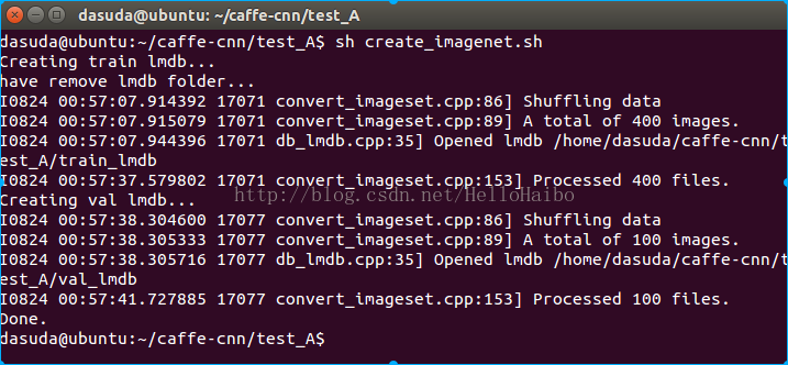

说明生成成功，如果不成功呢，十有八九时路径问题，你可以根据错误提示自己排查一下。

接下来，你会在同级目录下发现两个新文件夹train_lmdb和val_lmdb：

这两个文件夹里都是一个data.mdb和lock.mdb，data.mdb较大80多M。

到这一步，ok，lmdb文件生成结束，简单吧，接下来生成均值文件更简单。

二、生成均值文件

均值文件时训练网络时候必不可少的文件，会提高训练速度和精度，网络中的操作时对于读取的图片都减去均值。

用样我们生成均值文件是使用caffe的工具compute_image_mean，脚本如下：

[python] view plain copy

1. <span style="font-size:18px;">#!/usr/bin/env sh  
2. #以下三个路径跟生成lmdb脚本中的一致，可以直接copy过来  
3. EXAMPLE=/home/dasuda/caffe-cnn/test_A   
4. DATA=/home/dasuda/caffe-cnn/test_A  
5. TOOLS=/home/dasuda/caffe/tools  
6.   
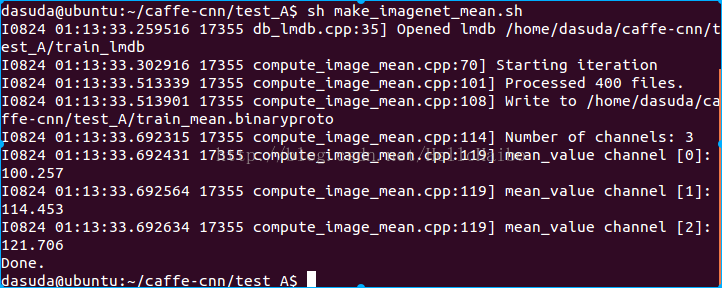
7. $TOOLS/compute_image_mean $EXAMPLE/train_lmdb \ #传人训练lmdb文件夹，注意这里只传入train_lmdb  
8.   $DATA/train_mean.binaryproto ￥生成的均值文件名称，后缀为binaryproto  
9.   
10. echo "Done."</span>  

我的实现方法

sudo build/tools/compute_image_mean mytest1/zhn/img_train_lmdb mytest1/mean.binaryproto

运行以上脚本后，出现：

说明生成成功，如果不成功呢，十有八九时路径问题，你可以根据错误提示自己排查一下。

在统计目录下即可看到生成的.binaryproto文件。

ok，至此，我们已经生成了训练模型的数据处理部分，下一篇我们将介绍如何编写模型结构文件和训练规则文件。

Caffe实战Day3-准备网络结构文件和训练文件（重点）

友情链接：我的caffe实战Day2-准备lmdb文件和均值文件

通过前两篇文章，我们已经把训练模型的数据准备好了，并做了需要做的预处理，接下来我们就开始准备网络结构文件，在开始之前呢，我们先列一下清单：

ok，本此我们就是准备其中的train_val.prototxt，deploy.prorotxt,solver.prototxt三个文件，最后的caffemodel文件，相信大家从名字也可以看出来，这个时训练成功后生成的模型参数文件，他涉及到模型的训练，我们放到下一篇来讲解。

一、train_val.prototxt

这个文件呢，是网络的结构文件，一般说设计网络，狭义上就是指的设计这个文件的内容，对于初学者，我建议你们先用简单的模板训练，在看懂的基础上，了解这个文件的结构，以及自己如何去设计这个文件。

caffe自带的demo中有很简单的，也很经典的LeNet、AlexNet、GoogLeNet模型(google为了向经典的LeNet致敬，才将L大写)，再次强烈建议大家将这些模型的结构看一遍，弄懂为何这样设计，这对你以后自己去设计网络有很大的启发，当然基本的数理统计算法，比如经典的BP算法、autoencoder、基本的激活函数sigmoid函数LRN函数等等，这些需要根据格个人情况自行补课。

好了，废话不多说，我们马上开始准备train_val.prototxt文件。

我们采用自带的CaffeNet为例，层数少，容易理解，将caffe/models/bvlc_reference_caffenet下的文件全都copy到你的工作目录下。像我一样我把这个文件夹复制到我的工作目录下，并重命名为make_model。

大家打开刚才复制的文件夹，其实三个文件我们都可以找到，我们先打开train_val.prototxt文件，代码如下：

[python] view plain copy

1. name: "CaffeNet"  
2. layer {  
3.   name: "data"  
4.   type: "Data"  
5.   top: "data"  
6.   top: "label"  
7.   include {  
8.     phase: TRAIN   
9.   }  
10.   transform_param {  
11.     mirror: true   
12.     crop_size: 227   
13.     mean_file: "/home/dasuda/caffe-cnn/test_A/train_mean.binaryproto" //这里是训练的均值文件  
14.   }  
15.   data_param {  
16.     source: "/home/dasuda/caffe-cnn/test_A/train_lmdb" //训练的数据库文件  
17.     batch_size: 32   #每次训练的熟练，这里说明每次训练32张图片  
18.     backend: LMDB #传入的文件格式为lmdb  
19.   }  
20. }  
21. layer {  
22.   name: "data"  
23.   type: "Data"  
24.   top: "data"  
25.   top: "label"  
26.   include {  
27.     phase: TEST  
28.   }  
29.   transform_param {  
30.     mirror: false  
31.     crop_size: 227  
32.     mean_file: "/home/dasuda/caffe-cnn/test_A/train_mean.binaryproto" #训练的均值文件  
33.   }  
34.   data_param {  
35.     source: "/home/dasuda/caffe-cnn/test_A/val_lmdb" //测试的数据库文件  
36.     batch_size: 50  //每次测试多少张，这个与solver文件里面的参数有关  
37.     backend: LMDB  
38.   }  
39. }  
40. layer {  
41.   name: "conv1"  
42.   type: "Convolution"  
43.   bottom: "data"  
44.   top: "conv1"  
45.   param {  
46.     lr_mult: 1  
47.     decay_mult: 1  
48.   }  
49.   param {  
50.     lr_mult: 2  
51.     decay_mult: 0  
52.   }  
53.   convolution_param {  
54.     num_output: 96  
55.     kernel_size: 11  
56.     stride: 4  
57.     weight_filler {  
58.       type: "gaussian"  
59.       std: 0.01  
60.     }  
61.     bias_filler {  
62.       type: "constant"  
63.       value: 0  
64.     }  
65.   }  
66. }  
67. layer {  
68.   name: "relu1"  
69.   type: "ReLU"  
70.   bottom: "conv1"  
71.   top: "conv1"  
72. }  
73. layer {  
74.   name: "pool1"  
75.   type: "Pooling"  
76.   bottom: "conv1"  
77.   top: "pool1"  
78.   pooling_param {  
79.     pool: MAX  
80.     kernel_size: 3  
81.     stride: 2  
82.   }  
83. }  
84. layer {  
85.   name: "norm1"  
86.   type: "LRN"  
87.   bottom: "pool1"  
88.   top: "norm1"  
89.   lrn_param {  
90.     local_size: 5  
91.     alpha: 0.0001  
92.     beta: 0.75  
93.   }  
94. }  
95. layer {  
96.   name: "conv2"  
97.   type: "Convolution"  
98.   bottom: "norm1"  
99.   top: "conv2"  
100.   param {  
101.     lr_mult: 1  
102.     decay_mult: 1  
103.   }  
104.   param {  
105.     lr_mult: 2  
106.     decay_mult: 0  
107.   }  
108.   convolution_param {  
109.     num_output: 256  
110.     pad: 2  
111.     kernel_size: 5  
112.     group: 2  
113.     weight_filler {  
114.       type: "gaussian"  
115.       std: 0.01  
116.     }  
117.     bias_filler {  
118.       type: "constant"  
119.       value: 1  
120.     }  
121.   }  
122. }  
123. layer {  
124.   name: "relu2"  
125.   type: "ReLU"  
126.   bottom: "conv2"  
127.   top: "conv2"  
128. }  
129. layer {  
130.   name: "pool2"  
131.   type: "Pooling"  
132.   bottom: "conv2"  
133.   top: "pool2"  
134.   pooling_param {  
135.     pool: MAX  
136.     kernel_size: 3  
137.     stride: 2  
138.   }  
139. }  
140. layer {  
141.   name: "norm2"  
142.   type: "LRN"  
143.   bottom: "pool2"  
144.   top: "norm2"  
145.   lrn_param {  
146.     local_size: 5  
147.     alpha: 0.0001  
148.     beta: 0.75  
149.   }  
150. }  
151. layer {  
152.   name: "conv3"  
153.   type: "Convolution"  
154.   bottom: "norm2"  
155.   top: "conv3"  
156.   param {  
157.     lr_mult: 1  
158.     decay_mult: 1  
159.   }  
160.   param {  
161.     lr_mult: 2  
162.     decay_mult: 0  
163.   }  
164.   convolution_param {  
165.     num_output: 384  
166.     pad: 1  
167.     kernel_size: 3  
168.     weight_filler {  
169.       type: "gaussian"  
170.       std: 0.01  
171.     }  
172.     bias_filler {  
173.       type: "constant"  
174.       value: 0  
175.     }  
176.   }  
177. }  
178. layer {  
179.   name: "relu3"  
180.   type: "ReLU"  
181.   bottom: "conv3"  
182.   top: "conv3"  
183. }  
184. layer {  
185.   name: "conv4"  
186.   type: "Convolution"  
187.   bottom: "conv3"  
188.   top: "conv4"  
189.   param {  
190.     lr_mult: 1  
191.     decay_mult: 1  
192.   }  
193.   param {  
194.     lr_mult: 2  
195.     decay_mult: 0  
196.   }  
197.   convolution_param {  
198.     num_output: 384  
199.     pad: 1  
200.     kernel_size: 3  
201.     group: 2  
202.     weight_filler {  
203.       type: "gaussian"  
204.       std: 0.01  
205.     }  
206.     bias_filler {  
207.       type: "constant"  
208.       value: 1  
209.     }  
210.   }  
211. }  
212. layer {  
213.   name: "relu4"  
214.   type: "ReLU"  
215.   bottom: "conv4"  
216.   top: "conv4"  
217. }  
218. layer {  
219.   name: "conv5"  
220.   type: "Convolution"  
221.   bottom: "conv4"  
222.   top: "conv5"  
223.   param {  
224.     lr_mult: 1  
225.     decay_mult: 1  
226.   }  
227.   param {  
228.     lr_mult: 2  
229.     decay_mult: 0  
230.   }  
231.   convolution_param {  
232.     num_output: 256  
233.     pad: 1  
234.     kernel_size: 3  
235.     group: 2  
236.     weight_filler {  
237.       type: "gaussian"  
238.       std: 0.01  
239.     }  
240.     bias_filler {  
241.       type: "constant"  
242.       value: 1  
243.     }  
244.   }  
245. }  
246. layer {  
247.   name: "relu5"  
248.   type: "ReLU"  
249.   bottom: "conv5"  
250.   top: "conv5"  
251. }  
252. layer {  
253.   name: "pool5"  
254.   type: "Pooling"  
255.   bottom: "conv5"  
256.   top: "pool5"  
257.   pooling_param {  
258.     pool: MAX  
259.     kernel_size: 3  
260.     stride: 2  
261.   }  
262. }  
263. layer {  
264.   name: "fc6"  
265.   type: "InnerProduct"  
266.   bottom: "pool5"  
267.   top: "fc6"  
268.   param {  
269.     lr_mult: 1  
270.     decay_mult: 1  
271.   }  
272.   param {  
273.     lr_mult: 2  
274.     decay_mult: 0  
275.   }  
276.   inner_product_param {  
277.     num_output: 4096  
278.     weight_filler {  
279.       type: "gaussian"  
280.       std: 0.005  
281.     }  
282.     bias_filler {  
283.       type: "constant"  
284.       value: 1  
285.     }  
286.   }  
287. }  
288. layer {  
289.   name: "relu6"  
290.   type: "ReLU"  
291.   bottom: "fc6"  
292.   top: "fc6"  
293. }  
294. layer {  
295.   name: "drop6"  
296.   type: "Dropout"  
297.   bottom: "fc6"  
298.   top: "fc6"  
299.   dropout_param {  
300.     dropout_ratio: 0.5  
301.   }  
302. }  
303. layer {  
304.   name: "fc7"  
305.   type: "InnerProduct"  
306.   bottom: "fc6"  
307.   top: "fc7"  
308.   param {  
309.     lr_mult: 1  
310.     decay_mult: 1  
311.   }  
312.   param {  
313.     lr_mult: 2  
314.     decay_mult: 0  
315.   }  
316.   inner_product_param {  
317.     num_output: 4096  
318.     weight_filler {  
319.       type: "gaussian"  
320.       std: 0.005  
321.     }  
322.     bias_filler {  
323.       type: "constant"  
324.       value: 1  
325.     }  
326.   }  
327. }  
328. layer {  
329.   name: "relu7"  
330.   type: "ReLU"  
331.   bottom: "fc7"  
332.   top: "fc7"  
333. }  
334. layer {  
335.   name: "drop7"  
336.   type: "Dropout"  
337.   bottom: "fc7"  
338.   top: "fc7"  
339.   dropout_param {  
340.     dropout_ratio: 0.5  
341.   }  
342. }  
343. layer {  
344.   name: "fc8"  
345.   type: "InnerProduct"  
346.   bottom: "fc7"  
347.   top: "fc8"  
348.   param {  
349.     lr_mult: 1  
350.     decay_mult: 1  
351.   }  
352.   param {  
353.     lr_mult: 2  
354.     decay_mult: 0  
355.   }  
356.   inner_product_param {  
357.     num_output: 5 #这个时最后一层全连接层，这个参数说明你要输出的类别数，我们这里有五类图片，故值为5  
358.     weight_filler {  
359.       type: "gaussian"  
360.       std: 0.01  
361.     }  
362.     bias_filler {  
363.       type: "constant"  
364.       value: 0  
365.     }  
366.   }  
367. }  
368. layer {  
369.   name: "accuracy"  
370.   type: "Accuracy"  
371.   bottom: "fc8"  
372.   bottom: "label"  
373.   top: "accuracy"  
374.   include {  
375.     phase: TEST  
376.   }  
377. }  
378. layer {  
379.   name: "loss"  
380.   type: "SoftmaxWithLoss"  
381.   bottom: "fc8"  
382.   bottom: "label"  
383.   top: "loss"  
384. }  

这个文件只需要修改我注释的地方，一共三层，两层输入，一层输出，中间的可以不用修改。后面我会写一篇关于train_val.prototxt详解的文章。

通过修改大家可以看出来，这个网络需要输入1、数据库文件，两个lmdb文件，一个训练一个测试。2、均值文件，加快训练速度，提高训练精度。网络输出：（训练情况下）loss rate和accuracy rate，一个是在训练集上的准确度，越小越好，说明网络的输出与标签“差距”很小，并且网络就是通过这个损失函数来改变各个参数的大小，达到学习的效果。第二个时测试集上的准确度，越大越好。

二、deploy.prototxt文件

这个文件是根据train_val.prototxt编写的，里面结构大体一样，只是把训练的参数去掉。

这个文件我们只需要修改一处，将输出的类别改为5

代码如下：

[python] view plain copy

1. name: "CaffeNet"  
2. layer {  
3.   name: "data"  
4.   type: "Input"  
5.   top: "data"  
6.   input_param { shape: { dim: 10 dim: 3 dim: 227 dim: 227 } }  
7. }  
8. layer {  
9.   name: "conv1"  
10.   type: "Convolution"  
11.   bottom: "data"  
12.   top: "conv1"  
13.   convolution_param {  
14.     num_output: 96  
15.     kernel_size: 11  
16.     stride: 4  
17.   }  
18. }  
19. layer {  
20.   name: "relu1"  
21.   type: "ReLU"  
22.   bottom: "conv1"  
23.   top: "conv1"  
24. }  
25. layer {  
26.   name: "pool1"  
27.   type: "Pooling"  
28.   bottom: "conv1"  
29.   top: "pool1"  
30.   pooling_param {  
31.     pool: MAX  
32.     kernel_size: 3  
33.     stride: 2  
34.   }  
35. }  
36. layer {  
37.   name: "norm1"  
38.   type: "LRN"  
39.   bottom: "pool1"  
40.   top: "norm1"  
41.   lrn_param {  
42.     local_size: 5  
43.     alpha: 0.0001  
44.     beta: 0.75  
45.   }  
46. }  
47. layer {  
48.   name: "conv2"  
49.   type: "Convolution"  
50.   bottom: "norm1"  
51.   top: "conv2"  
52.   convolution_param {  
53.     num_output: 256  
54.     pad: 2  
55.     kernel_size: 5  
56.     group: 2  
57.   }  
58. }  
59. layer {  
60.   name: "relu2"  
61.   type: "ReLU"  
62.   bottom: "conv2"  
63.   top: "conv2"  
64. }  
65. layer {  
66.   name: "pool2"  
67.   type: "Pooling"  
68.   bottom: "conv2"  
69.   top: "pool2"  
70.   pooling_param {  
71.     pool: MAX  
72.     kernel_size: 3  
73.     stride: 2  
74.   }  
75. }  
76. layer {  
77.   name: "norm2"  
78.   type: "LRN"  
79.   bottom: "pool2"  
80.   top: "norm2"  
81.   lrn_param {  
82.     local_size: 5  
83.     alpha: 0.0001  
84.     beta: 0.75  
85.   }  
86. }  
87. layer {  
88.   name: "conv3"  
89.   type: "Convolution"  
90.   bottom: "norm2"  
91.   top: "conv3"  
92.   convolution_param {  
93.     num_output: 384  
94.     pad: 1  
95.     kernel_size: 3  
96.   }  
97. }  
98. layer {  
99.   name: "relu3"  
100.   type: "ReLU"  
101.   bottom: "conv3"  
102.   top: "conv3"  
103. }  
104. layer {  
105.   name: "conv4"  
106.   type: "Convolution"  
107.   bottom: "conv3"  
108.   top: "conv4"  
109.   convolution_param {  
110.     num_output: 384  
111.     pad: 1  
112.     kernel_size: 3  
113.     group: 2  
114.   }  
115. }  
116. layer {  
117.   name: "relu4"  
118.   type: "ReLU"  
119.   bottom: "conv4"  
120.   top: "conv4"  
121. }  
122. layer {  
123.   name: "conv5"  
124.   type: "Convolution"  
125.   bottom: "conv4"  
126.   top: "conv5"  
127.   convolution_param {  
128.     num_output: 256  
129.     pad: 1  
130.     kernel_size: 3  
131.     group: 2  
132.   }  
133. }  
134. layer {  
135.   name: "relu5"  
136.   type: "ReLU"  
137.   bottom: "conv5"  
138.   top: "conv5"  
139. }  
140. layer {  
141.   name: "pool5"  
142.   type: "Pooling"  
143.   bottom: "conv5"  
144.   top: "pool5"  
145.   pooling_param {  
146.     pool: MAX  
147.     kernel_size: 3  
148.     stride: 2  
149.   }  
150. }  
151. layer {  
152.   name: "fc6"  
153.   type: "InnerProduct"  
154.   bottom: "pool5"  
155.   top: "fc6"  
156.   inner_product_param {  
157.     num_output: 4096  
158.   }  
159. }  
160. layer {  
161.   name: "relu6"  
162.   type: "ReLU"  
163.   bottom: "fc6"  
164.   top: "fc6"  
165. }  
166. layer {  
167.   name: "drop6"  
168.   type: "Dropout"  
169.   bottom: "fc6"  
170.   top: "fc6"  
171.   dropout_param {  
172.     dropout_ratio: 0.5  
173.   }  
174. }  
175. layer {  
176.   name: "fc7"  
177.   type: "InnerProduct"  
178.   bottom: "fc6"  
179.   top: "fc7"  
180.   inner_product_param {  
181.     num_output: 4096  
182.   }  
183. }  
184. layer {  
185.   name: "relu7"  
186.   type: "ReLU"  
187.   bottom: "fc7"  
188.   top: "fc7"  
189. }  
190. layer {  
191.   name: "drop7"  
192.   type: "Dropout"  
193.   bottom: "fc7"  
194.   top: "fc7"  
195.   dropout_param {  
196.     dropout_ratio: 0.5  
197.   }  
198. }  
199. layer {  
200.   name: "fc8"  
201.   type: "InnerProduct"  
202.   bottom: "fc7"  
203.   top: "fc8"  
204.   inner_product_param {  
205.     num_output: 5 #输出的类别  
206.   }  
207. }  
208. layer {  
209.   name: "prob"  
210.   type: "Softmax"  
211.   bottom: "fc8"  
212.   top: "prob"  
213. }  

好了至此，网络结构已经搭建好了，还时那句话，难点在train_val.prototxt文件的编写，这里我们只是参考了现成的简单的网络。

三、solver.prototxt

这个文件就是配置一下训练时的规则，这个文件里面的参数也是模型质量的关键。（我会单独写一篇文章去讲解这个文件）

[python] view plain copy

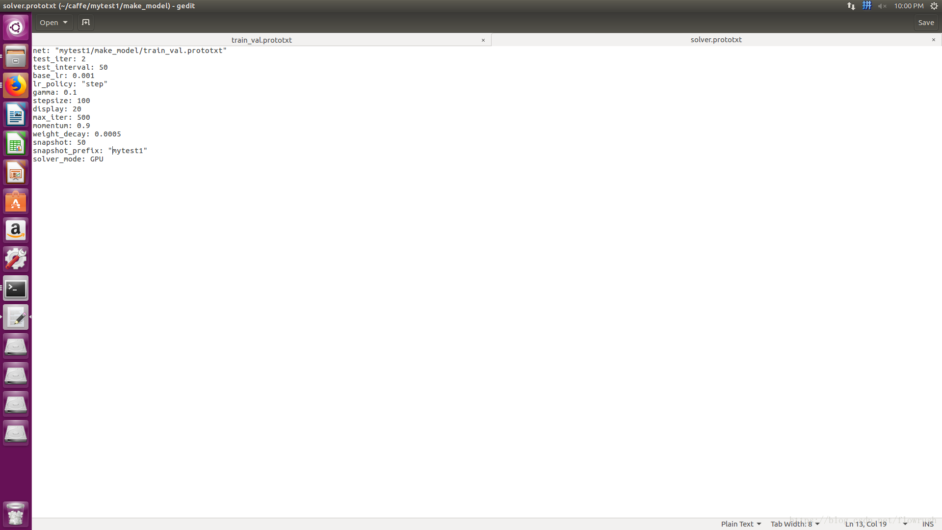
1. net: "/home/dasuda/caffe-cnn/test_A/make_model/train_val.prototxt" #这里时train_val.prototxt文件的路径  把/home/dasuda/caffe-cnn/去掉
2. test_iter: 2 #这个值乘以train_val.prototxt中第二个layer里面的batch_size等与你训练集的大小，我这里时50*2=100  
3. test_interval: 50  
4. base_lr: 0.001 #学习率  
5. lr_policy: "step"  
6. gamma: 0.1   
7. stepsize: 100  
8. display: 20  
9. max_iter: 500 #最大训练次数  
10. momentum: 0.9  
11. weight_decay: 0.0005  
12. snapshot: 50 #每50次保存一次模型快照，以便中断训练时继续训练，也可以  
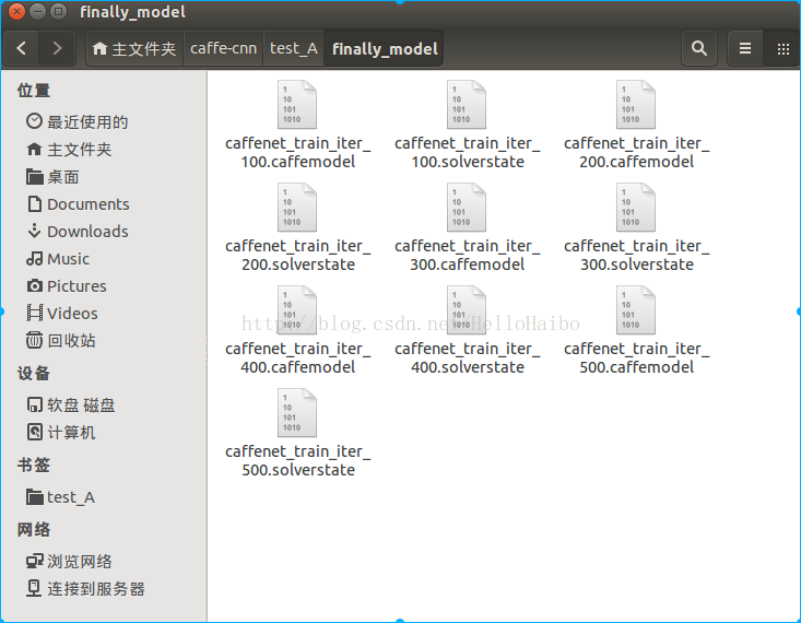
13. snapshot_prefix: "/home/dasuda/caffe-cnn/test_A/finally_model/caffenet_train" #生成快照的路径  
14. solver_mode: CPU #训练的模式  

ok，三个文件已经准备好了，至此，训练模型的所有文件都已经准备好了，下一篇我们将开始训练模型。

Caffe实战Day4-开始模型训练

OK，我们已经来到了最后一步-模型的训练，前三篇文章，我们已经将训练模型所需的文件、数据都准备好了，接下来一条命令就可开始模型的训练。

新建脚本或者你也可以直接输入命令：

[python] view plain copy

1. #!/usr/bin/env sh  
2. /home/dasuda/caffe/build/tools/caffe train \  
3.     --solver=/home/dasuda/caffe-cnn/test_A/make_model/solver.prototxt  

其中第一行是调用了caffe的工具train命令，第二行开头的参数--solver说明接下来是调用solver文件，后面跟你的solver文件路径即可，建议路径全部使用绝对路径。
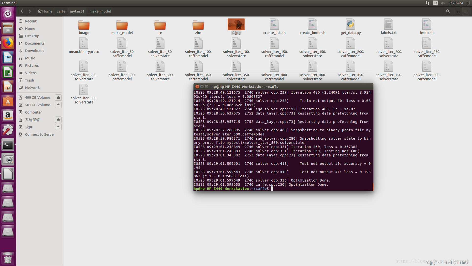
运行脚本后：

[plain] view plain copy

1. I0829 19:47:28.209851  3457 layer_factory.hpp:77] Creating layer data  
2. I0829 19:47:28.266258  3457 db_lmdb.cpp:35] Opened lmdb /home/dasuda/caffe-cnn/test_A/train_lmdb  
3. I0829 19:47:28.286499  3457 net.cpp:84] Creating Layer data  
4. I0829 19:47:28.286763  3457 net.cpp:380] data -> data  
5. I0829 19:47:28.288883  3457 net.cpp:380] data -> label  
6. I0829 19:47:28.288946  3457 data_transformer.cpp:25] Loading mean file from: /home/dasuda/caffe-cnn/test_A/train_mean.binaryproto  
7. I0829 19:47:28.314162  3457 data_layer.cpp:45] output data size: 32,3,227,227  
8. I0829 19:47:28.657215  3457 net.cpp:122] Setting up data  
9. I0829 19:47:28.657289  3457 net.cpp:129] Top shape: 32 3 227 227 (4946784)  
10. I0829 19:47:28.657311  3457 net.cpp:129] Top shape: 32 (32)  
11. I0829 19:47:28.657333  3457 net.cpp:137] Memory required for data: 19787264  
12. I0829 19:47:28.657356  3457 layer_factory.hpp:77] Creating layer conv1  
13. I0829 19:47:28.657395  3457 net.cpp:84] Creating Layer conv1  
14. I0829 19:47:28.657428  3457 net.cpp:406] conv1 <- data  
15. I0829 19:47:28.657459  3457 net.cpp:380] conv1 -> conv1  
16. I0829 19:47:28.663385  3457 net.cpp:122] Setting up conv1  
17. I0829 19:47:28.663475  3457 net.cpp:129] Top shape: 32 96 55 55 (9292800)  
18. I0829 19:47:28.663489  3457 net.cpp:137] Memory required for data: 56958464  
19. I0829 19:47:28.663663  3457 layer_factory.hpp:77] Creating layer relu1  
20. I0829 19:47:28.663693  3457 net.cpp:84] Creating Layer relu1  
21. I0829 19:47:28.663720  3457 net.cpp:406] relu1 <- conv1  
22. I0829 19:47:28.663738  3457 net.cpp:367] relu1 -> conv1 (in-place)  
23. I0829 19:47:28.664847  3457 net.cpp:122] Setting up relu1  
24. I0829 19:47:28.664887  3457 net.cpp:129] Top shape: 32 96 55 55 (9292800)  
25. I0829 19:47:28.664894  3457 net.cpp:137] Memory required for data: 94129664  
26. I0829 19:47:28.664899  3457 layer_factory.hpp:77] Creating layer pool1  
27. I0829 19:47:28.664932  3457 net.cpp:84] Creating Layer pool1  
28. I0829 19:47:28.664980  3457 net.cpp:406] pool1 <- conv1  
29. I0829 19:47:28.665011  3457 net.cpp:380] pool1 -> pool1  
30. I0829 19:47:28.665050  3457 net.cpp:122] Setting up pool1  
31. I0829 19:47:28.665076  3457 net.cpp:129] Top shape: 32 96 27 27 (2239488)  
32. I0829 19:47:28.665087  3457 net.cpp:137] Memory required for data: 103087616  
33. I0829 19:47:28.665094  3457 layer_factory.hpp:77] Creating layer norm1  
34. I0829 19:47:28.665136  3457 net.cpp:84] Creating Layer norm1  
35. I0829 19:47:28.665164  3457 net.cpp:406] norm1 <- pool1  
36. I0829 19:47:28.665223  3457 net.cpp:380] norm1 -> norm1  
37. I0829 19:47:28.665256  3457 net.cpp:122] Setting up norm1  
38. I0829 19:47:28.665285  3457 net.cpp:129] Top shape: 32 96 27 27 (2239488)  
39. I0829 19:47:28.665310  3457 net.cpp:137] Memory required for data: 112045568  
40. I0829 19:47:28.665323  3457 layer_factory.hpp:77] Creating layer conv2  
41. I0829 19:47:28.665351  3457 net.cpp:84] Creating Layer conv2  

这一部分是创建输入层，也就是之前修改的data层，这里面包含一些重要的信息，比如当前层接受多大的数据，当前层的名称，当前训练阶段预计需要多大的内存等等。

[plain] view plain copy

1. I0829 19:47:48.050531  3457 solver.cpp:397]     Test net output #0: accuracy = 0.2  
2. I0829 19:47:48.050607  3457 solver.cpp:397]     Test net output #1: loss = 1.69832 (* 1 = 1.69832 loss)  
3. I0829 19:47:59.574867  3457 solver.cpp:218] Iteration 0 (-1.4013e-45 iter/s, 25.163s/20 iters), loss = 2.14062  
4. I0829 19:47:59.575369  3457 solver.cpp:237]     Train net output #0: loss = 2.14062 (* 1 = 2.14062 loss)  
5. I0829 19:47:59.575387  3457 sgd_solver.cpp:105] Iteration 0, lr = 0.001  
6. I0829 19:49:30.509104  3460 data_layer.cpp:73] Restarting data prefetching from start.  
7. I0829 19:51:40.608665  3457 solver.cpp:218] Iteration 20 (0.0904842 iter/s, 221.033s/20 iters), loss = 3.89005  
8. I0829 19:51:40.608927  3457 solver.cpp:237]     Train net output #0: loss = 3.89005 (* 1 = 3.89005 loss)  
9. I0829 19:51:40.608942  3457 sgd_solver.cpp:105] Iteration 20, lr = 0.001  

当然它还会输出当前一组训练数据到达输出层时，训练的loss，测试的accuracy，以及参数更新情况。

[plain] view plain copy

1. I0829 20:05:52.601330  3457 solver.cpp:447] Snapshotting to binary proto file /home/dasuda/caffe-cnn/test_A/finally_model/caffenet_train_iter_100.caffemodel  
2. I0829 20:06:02.162716  3457 sgd_solver.cpp:273] Snapshotting solver state to binary proto file /home/dasuda/caffe-cnn/test_A/finally_model/caffenet_train_iter_100.solverstate  

以上信息是说明，正在保存快照，快照时两部分，一个是caffenet_train_iter_(当前训练的数量).caffemodel，一个是caffenet_train_iter_(当前训练的数量).solverstate，第一个文件时模型文件，我们到时候可以直接使用500次时候的模型文件，第二个文件可以在你训练中断时，继续从当前位置开始训练。
对于我来说，我用的虚拟机，CPU训练，大概需要1个半小时：

[plain] view plain copy

1. I0829 21:16:03.929659  3457 sgd_solver.cpp:105] Iteration 480, lr = 1e-07  
2. I0829 21:16:34.835683  3460 data_layer.cpp:73] Restarting data prefetching from start.  
3. I0829 21:18:37.894023  3460 data_layer.cpp:73] Restarting data prefetching from start.  
4. I0829 21:19:19.841223  3457 solver.cpp:447] Snapshotting to binary proto file /home/dasuda/caffe-cnn/test_A/finally_model/caffenet_train_iter_500.caffemodel  
5. I0829 21:19:22.285903  3457 sgd_solver.cpp:273] Snapshotting solver state to binary proto file /home/dasuda/caffe-cnn/test_A/finally_model/caffenet_train_iter_500.solverstate  
6. I0829 21:19:28.835945  3457 solver.cpp:310] Iteration 500, loss = 0.143794  
7. I0829 21:19:28.836014  3457 solver.cpp:330] Iteration 500, Testing net (#0)  
8. I0829 21:19:28.877216  3463 data_layer.cpp:73] Restarting data prefetching from start.  
9. I0829 21:19:40.881701  3457 solver.cpp:397]     Test net output #0: accuracy = 0.94  
10. I0829 21:19:40.881819  3457 solver.cpp:397]     Test net output #1: loss = 0.232396 (* 1 = 0.232396 loss)  
11. I0829 21:19:40.881839  3457 solver.cpp:315] Optimization Done.  
12. I0829 21:19:40.881863  3457 caffe.cpp:259] Optimization Done.  

这就说明训练完成，在finally_model文件夹下就可以找到训练好的模型及快照：

注意：前面生成txt的label一定要从零开始，不然可能会出现loss=87.33情况。还有输出一定要改成你需要的。

其中caffenet_train_iter_500.caffemodel就是最终训练好的模型参数文件。

下面我们开始测试我们训练的网络：
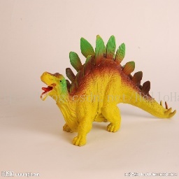
从网上找到一张恐龙的照片命名为test0.jpg

然后cd到caffe/example/cpp_classification输入以下命令：
sudo ./classification.bin /home/dasuda/caffe-cnn/test_A/make_model/deploy.prototxt /home/dasuda/caffe-cnn/test_A/finally_model/caffenet_train_iter_500.caffemodel /home/dasuda/caffe-cnn/test_A/train_mean.binaryproto /home/dasuda/caffe-cnn/test_A/labels.txt /home/dasuda/caffe-cnn/test_A/test0.jpg
其中./classification.bin为当前目录下的一个文件，是官方提供的C++接口，是用来测试的，后面跟了5个参数分别是：网络结构文件，训练的模型参数文件，均值文件，标签文件，测试图片

标签文件格式：
新建txt文档labels.txt
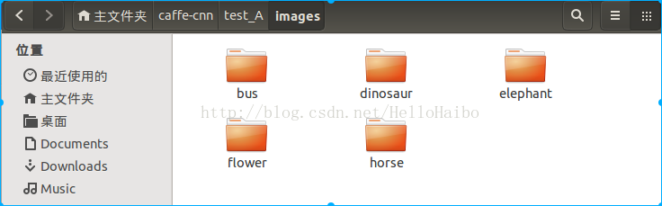
0 bus
1 dinosaur
2 elephant
3 flower
4 horse

即序号和你之前的训练数据标签一致，至于后面的英文名称是方面你测试的。

预测输出：

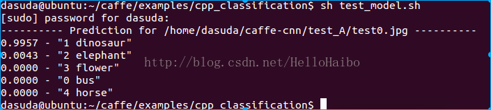
可见网络输出99.57%是恐龙，符合预期。

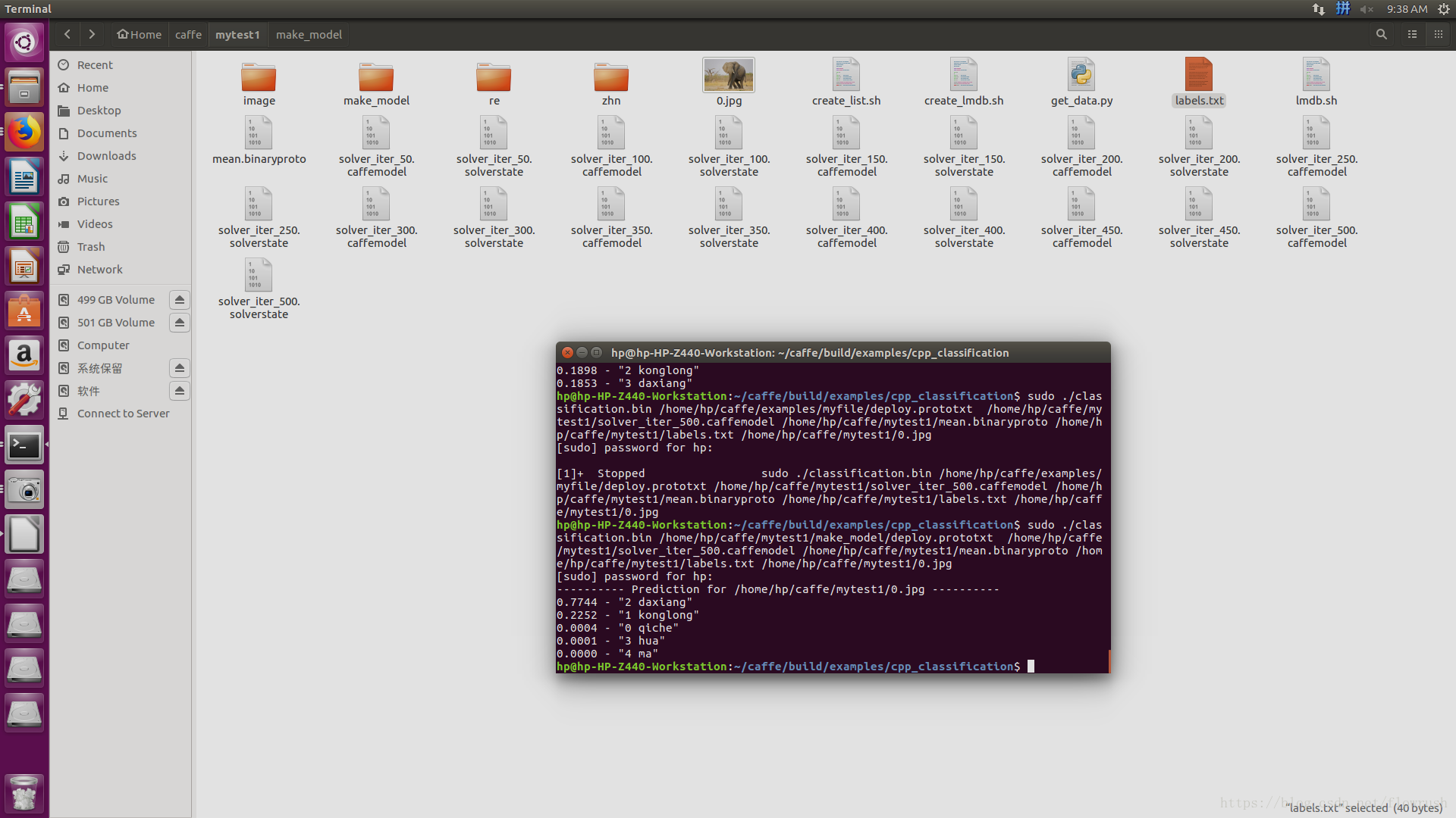
下面附上我的代码于结果

sudo ./classification.bin /home/hp/caffe/examples/myfile/deploy.prototxt  /home/hp/caffe/mytest1/solver_iter_500.caffemodel /home/hp/caffe/mytest1/mean.binaryproto /home/hp/caffe/mytest1/labels.txt /home/hp/caffe/mytest1/0.jpg

至此caffe入门到此结束，相信大家通过本系列文章的实践，对caffe训练网络的整个流程有了大体的认识，接下来大家需要多读paper，对模型搭建的某一步骤展开针对性的学习，并及时补充基础知识，相信功夫不负有心人，大家一定会收获预期的效果，谢谢大家。

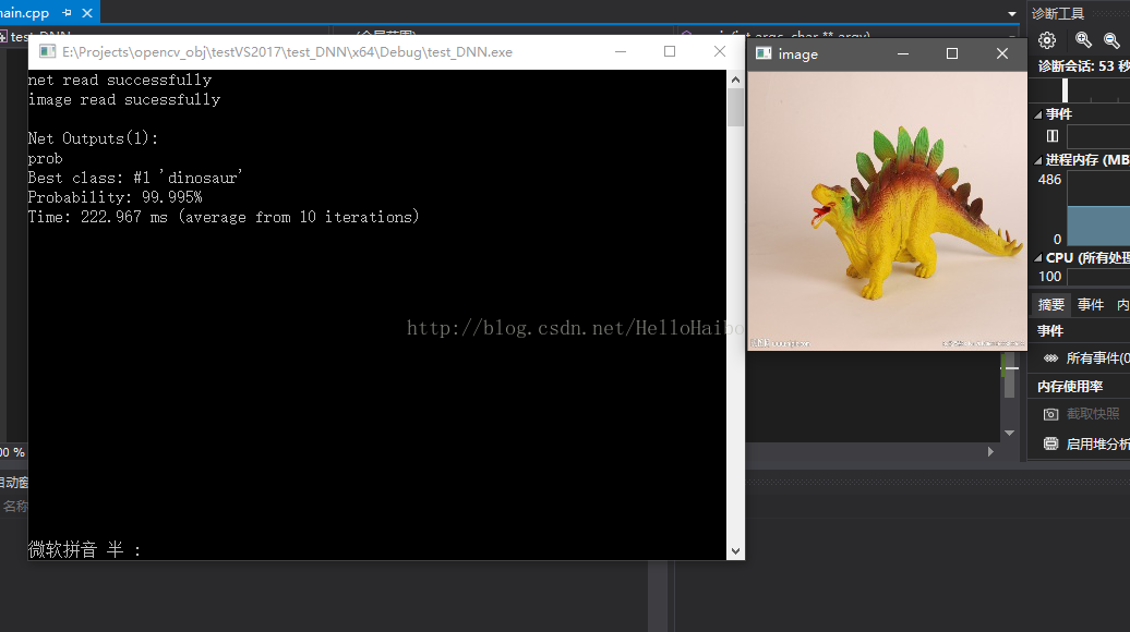
Caffe实战Day5-使用opencv调用caffe模型进行分类

通过前面的文章，我们已经使用caffe训练了一个模型，下面我们在opencv中使用模型进行预测吧！
环境：OpenCV 3.3+VS2017
准备好三个文件：deploy.prototxt、caffemdel文件、标签文件labels.txt，建议大家按照前面的文章生成相应的文件，因为格式不同，可能程序运行会有错误。
1、修改deploy.prototxt文件
只需将输入层的格式修改一下：

将

[plain] view plain copy

1. name: "CaffeNet"  
2. layer {  
3.   name: "data"  
4.   type: "Input"  
5.   top: "data"  
6.   input_param { shape: { dim: 10 dim: 3 dim: 227 dim: 227 } }  
7. }  

修改为:

[plain] view plain copy

1. name: "CaffeNet"  
2. input: "data"  
3. input_dim: 10   
4. input_dim: 3   
5. input_dim: 227   
6. input_dim: 227  

即可。
2、我将三个文件命名为：caffenet.prototxt、caffenet.caffemodel、labels.txt
3、VS新建工程，复制下面代码：

[cpp] view plain copy

1. #include <opencv2/dnn.hpp>  
2. #include <opencv2/imgproc.hpp>  
3. #include <opencv2/highgui.hpp>  
4. #include <opencv2/core/utils/trace.hpp>  
5. using namespace cv;  
6. using namespace cv::dnn;  
7.   
8. #include <fstream>  
9. #include <iostream>  
10. #include <cstdlib>  
11. using namespace std;  
12.   
13. //寻找出概率最高的一类  
14. static void getMaxClass(const Mat &probBlob, int *classId, double *classProb)  
15. {  
16.     Mat probMat = probBlob.reshape(1, 1);  
17.     Point classNumber;  
18.   
19.     minMaxLoc(probMat, NULL, classProb, NULL, &classNumber);  
20.     *classId = classNumber.x;  
21. }  
22. //从标签文件读取分类 空格为标志  
23. static std::vector<String> readClassNames(const char *filename = "labels.txt")  
24. {  
25.     std::vector<String> classNames;  
26.   
27.     std::ifstream fp(filename);  
28.     if (!fp.is_open())  
29.     {  
30.         std::cerr << "File with classes labels not found: " << filename << std::endl;  
31.         exit(-1);  
32.     }  
33.   
34.     std::string name;  
35.     while (!fp.eof())  
36.     {  
37.         std::getline(fp, name);  
38.         if (name.length())  
39.             classNames.push_back(name.substr(name.find(' ') + 1));  
40.     }  
41.     fp.close();  
42.     return classNames;  
43. }  
44. //主程序  
45. int main(int argc, char **argv)  
46. {  
47.     //初始化  
48.     CV_TRACE_FUNCTION();  
49.     //读取模型参数和模型结构文件  
50.     String modelTxt = "caffenet.prototxt";  
51.     String modelBin = "caffenet.caffemodel";  
52.     //读取图片  
53.     String imageFile = (argc > 1) ? argv[1] : "test0.jpg";  
54.   
55.     //合成网络  
56.     Net net = dnn::readNetFromCaffe(modelTxt, modelBin);  
57.     //判断网络是否生成成功  
58.     if (net.empty())  
59.     {  
60.         std::cerr << "Can't load network by using the following files: " << std::endl;  
61.         exit(-1);  
62.     }  
63.     cerr << "net read successfully" << endl;  
64.   
65.     //读取图片  
66.     Mat img = imread(imageFile);  
67.     imshow("image", img);  
68.     if (img.empty())  
69.     {  
70.         std::cerr << "Can't read image from the file: " << imageFile << std::endl;  
71.         exit(-1);  
72.     }  
73.     cerr << "image read sucessfully" << endl;  
74.   
75. /*  Mat inputBlob = blobFromImage(img, 1, Size(224, 224), 
76.                                     Scalar(104, 117, 123)); */   
77.   
78.     //构造blob，为传入网络做准备，图片不能直接进入网络  
79.     Mat inputBlob = blobFromImage(img, 1, Size(227, 227));  
80.       
81.     Mat prob;  
82.     cv::TickMeter t;  
83.     for (int i = 0; i < 10; i++)  
84.     {  
85.         CV_TRACE_REGION("forward");  
86.         //将构建的blob传入网络data层  
87.         net.setInput(inputBlob,"data");   
88.         //计时  
89.         t.start();  
90.         //前向预测  
91.         prob = net.forward("prob");    
92.         //停止计时  
93.         t.stop();  
94.     }  
95.   
96.     int classId;  
97.     double classProb;  
98.     //找出最高的概率ID存储在classId，对应的标签在classProb中  
99.     getMaxClass(prob, &classId, &classProb);  
100.   
101.     //打印出结果  
102.     std::vector<String> classNames = readClassNames();  
103.     std::cout << "Best class: #" << classId << " '" << classNames.at(classId) << "'" << std::endl;  
104.     std::cout << "Probability: " << classProb * 100 << "%" << std::endl;  
105.     //打印出花费时间  
106.     std::cout << "Time: " << (double)t.getTimeMilli() / t.getCounter() << " ms (average from " << t.getCounter() << " iterations)" << std::endl;  
107.   
108.     //便于观察结果  
109.     waitKey(0);  
110.     return 0;  
111. }   

4、运行程序得到下面结果：

OK，输出上述信息，就说明你的模型在opencv中调用没问题了，接下来就是深入学习网络结构，理解各种参数，学习各种框架，从中总结。希望大家戒骄戒躁，都能达到自己的目标，谢谢大家。