AlexNet文献阅读05

6结果

“6 Results” (Krizhevsky 等, 2017, p. 7)

“Our results on ILSVRC-2010 are summarized in Table 1. Our network achieves top-1 and top-5 test set error rates of 37.5% and 17.0%5. The best performance achieved during the ILSVRC2010 competition was 47.1% and 28.2% with an approach that averages the predictions produced from six sparse-coding models trained on different features [2], and since then the best published results are 45.7% and 25.7% with an approach that averages the predictions of two classifiers trained on Fisher Vectors (FVs) computed from two types of densely-sampled features [24].” (Krizhevsky 等, 2017, p. 7)

我们在ILSVRC - 2010上的结果总结在表1中。我们的网络实现了前1和前5测试集的错误率为37.5 %和17.0 % 。在ILSVRC2010竞赛中取得的最好成绩是47.1 %和28.2 %，其方法是将在不同特征上训练的六个稀疏编码模型的预测结果取平均值[ 2 ]，此后发表的最好结果是45.7 %和25.7 %，其方法是将从两类密集采样特征计算的Fisher向量( FV )上训练的两个分类器的预测结果取平均值[ 24 ]。

解读

(1)我们使用卷积神经网络取得前1和前5测试集的错误率为37.5 %和17.0 %。

(2)在之前取得的最好成绩是47.1%和28.2%，采用机器学习的稀疏编码模型在不同特征上进行训练取的平均值

(3)此后发表的最好结果是45.7 %和25.7 %,使用的是机器学习，从密集采样特征计算Fisher向量，取平均结果

“We also entered our model in the ILSVRC-2012 competition and report our results in Table 2. Since the ILSVRC-2012 test set labels are not publicly available, we cannot report test error rates for all the models that we tried. In the remainder of this paragraph, we use validation and test error rates interchangeably because in our experience they do not differ by more than 0.1% (see Table 2). The CNN described in this paper achieves a top-5 error rate of 18.2%. Averaging the predictions of five similar CNNs gives an error rate of 16.4%.raining one CNN, with an extra sixth convolutional layer over the last pooling layer, to classify the entire ImageNet Fall 2011 release (15M images, 22K categories), and then “fine-tuning” it on ILSVRC-2012 gives an error rate of 16.6%. Averaging the predictions of two CNNs that were pre-trained on the entire Fall 2011 release with the aforementioned five CNNs gives an error rate of 15.3%. The second-best contest entry achieved an error rate of 26.2% with an approach that averages the predictions of several classifiers trained on FVs computed from different types of densely-sampled features [7].” (Krizhevsky 等, 2017, p. 7)

我们还在ILSVRC - 2012竞赛中输入了我们的模型，并在表2中报告了我们的结果。由于ILSVRC - 2012测试集标签不公开，我们无法报告我们尝试的所有模型的测试错误率。在本段的剩余部分，我们交替使用验证错误率和测试错误率，因为在我们的经验中，它们的差异不超过0.1 % (见表2)。本文描述的CNN取得了18.2 %的前五名错误率。将5个相似CNN的预测结果进行平均，得到的错误率为16.4 %。雨淋一个CNN，在最后一个池化层上增加一个第六个卷积层，对整个ImageNet Fall 2011发布的( 15M图像, 22K类别)进行分类，然后在ILSVRC - 2012上"微调"它，错误率为16.6 %。使用前述5个CNN对2011年秋季发布的整个数据集进行预训练的2个CNN的预测结果进行平均，误差率为15.3 %。第二个最好的竞赛条目达到了26.2 %的错误率，其方法是平均从不同类型的密集采样特征计算的FV上训练的几个分类器的预测[ 7 ]。

“Finally, we also report our error rates on the Fall 2009 version of ImageNet with 10,184 categories and 8.9 million images. On this dataset we follow the convention in the literature of using half of the images for training and half for testing. Since there is no established test set, our split necessarily differs from the splits used by previous authors, but this does not affect the results appreciably. Our top-1 and top-5 error rates on this dataset are 67.4% and 40.9%, attained by the net described above but with an additional, sixth convolutional layer over the last pooling layer. The best published results on this dataset are 78.1% and 60.9% [19].” (Krizhevsky 等, 2017, p. 7)

最后，我们还报告了我们在Fall2009版本的ImageNet上的错误率，共有10184个类别和890万张图像。在这个数据集上我们遵循文献中的约定，使用一半的图像用于训练，一半用于测试。由于没有既定的测试集，我们的拆分必然与之前作者使用的拆分有所不同，但这并不明显影响结果。我们在这个数据集上的top - 1和top - 5错误率分别为67.4 %和40.9 %，通过上面描述的网络，但在最后一个池化层上增加了第六个卷积层。在这个数据集上最好的公布结果是78.1 %和60.9 % [ 19 ]。

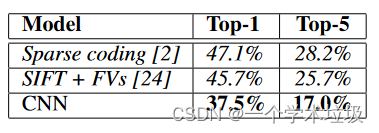
“Table 1: Comparison of results on ILSVRC2010 test set. In italics are best results achieved by others.” (Krizhevsky 等, 2017, p. 7) 表1：ILSVRC2010测试集上的结果对比。斜体字是别人取得的最好成绩。

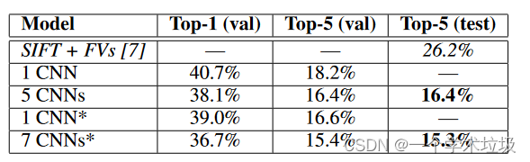
“Table 2: Comparison of error rates on ILSVRC-2012 validation and test sets. In italics are best results achieved by others. Models with an asterisk* were “pre-trained” to classify the entire ImageNet 2011 Fall release. See Section 6 for details.” (Krizhevsky 等, 2017, p. 7) 表2：ILSVRC - 2012验证集和测试集上的错误率比较。斜体字是别人取得的最好成绩。带有星号*的模型被"预训练"以分类整个ImageNet 2011 Fall版本。详见第6节。

“6.1 Qualitative Evaluations” (Krizhevsky 等, 2017, p. 7) 6.1定性评价

“Figure 3 shows the convolutional kernels learned by the network’s two data-connected layers. The network has learned a variety of frequency- and orientation-selective kernels, as well as various colored blobs. Notice the specialization exhibited by the two GPUs, a result of the restricted connectivity described in Section 3.5. The kernels on GPU 1 are largely color-agnostic, while the kernels on on GPU 2 are largely color-specific. This kind of specialization occurs during every run and is independent of any particular random weight initialization (modulo a renumbering of the GPUs).” (Krizhevsky 等, 2017, p. 7) 图3显示了网络的两个数据对接层学习到的卷积核。该网络学习了多种频率和方向选择性的核，以及各种颜色的斑点。注意到两个GPU所表现出的特殊化，这是3.5节中描述的限制连通性的结果。GPU 1上的内核主要是颜色无关的，而GPU 2上的内核主要是颜色相关的。这种专门化发生在每次运行期间，并且独立于任何特定的随机权重初始化(对GPU进行重新编号)。

解读

(1)由于神经网络连接的原因，从而使GPU1和GPU2表现2种不同，GPU1和颜色无关，GPU2和颜色相关

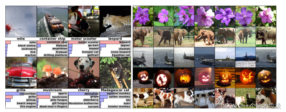
“Figure 4: (Left) Eight ILSVRC-2010 test images and the five labels considered most probable by our model. The correct label is written under each image, and the probability assigned to the correct label is also shown with a red bar (if it happens to be in the top 5). (Right) Five ILSVRC-2010 test images in the first column. The remaining columns show the six training images that produce feature vectors in the last hidden layer with the smallest Euclidean distance from the feature vector for the test image.” (Krizhevsky 等, 2017, p. 8) 图4：(左) 8幅ILSVRC - 2010测试图像和我们模型认为最有可能的5个标签。在每张图像下面写入正确的标签，分配给正确标签的概率也用红色条(如果恰好位于前5名)显示。(右)第一列5幅ILSVRC - 2010测试图像。剩余的列显示了在最后一个隐藏层中产生特征向量的6幅训练图像，这些训练图像与测试图像的特征向量的欧氏距离最小。

解读

(1)在最后一层隐藏层中，在语义空间里面表现的非常好

“In the left panel of Figure 4 we qualitatively assess what the network has learned by computing its top-5 predictions on eight test images. Notice that even off-center objects, such as the mite in the top-left, can be recognized by the net. Most of the top-5 labels appear reasonable. For example, only other types of cat are considered plausible labels for the leopard. In some cases (grille, cherry) there is genuine ambiguity about the intended focus of the photograph.” (Krizhevsky 等, 2017, p. 8) 在图4的左边面板中，我们定性地评估了网络通过在八张测试图像上计算其前5个预测所学习到的内容。注意，即使是偏离中心的对象，比如左上角的螨，也可以被网络识别。大多数前5个标签似乎是合理的。例如，只有其他类型的猫被认为是豹的标签。在某些情况下，(格栅,樱桃)对照片的预期焦点有真正的模糊性。

“Another way to probe the network’s visual knowledge is to consider the feature activations induced by an image at the last, 4096-dimensional hidden layer. If two images produce feature activation vectors with a small Euclidean separation, we can say that the higher levels of the neural network consider them to be similar. Figure 4 shows five images from the test set and the six images from the training set that are most similar to each of them according to this measure. Notice that at the pixel level, the retrieved training images are generally not close in L2 to the query images in the first column. For example, the retrieved dogs and elephants appear in a variety of poses. We present the results for many more test images in the supplementary material.” (Krizhevsky 等, 2017, p. 8) 探索网络视觉知识的另一种方法是考虑图像在最后一个4096维隐藏层引起的特征激活。如果两幅图像产生的特征激活向量具有很小的欧氏距离，我们可以说神经网络的较高级别认为它们是相似的。图4显示了来自测试集的五幅图像和来自训练集的六幅图像，它们与根据此度量得到的每幅图像最相似。注意，在像素级别上，检索到的训练图像在L2上一般与第1列的查询图像不接近。例如，检索到的狗和大象以多种姿态出现。我们在补充材料中展示了更多测试图像的结果。

解读

(1)欧氏距离越小，两者之间越接近

“Computing similarity by using Euclidean distance between two 4096-dimensional, real-valued vectors is inefficient, but it could be made efficient by training an auto-encoder to compress these vectors to short binary codes. This should produce a much better image retrieval method than applying autoencoders to the raw pixels [14], which does not make use of image labels and hence has a tendency to retrieve images with similar patterns of edges, whether or not they are semantically similar.” (Krizhevsky 等, 2017, p. 8) 使用两个4096维实值向量之间的欧氏距离计算相似性是低效的，但是可以通过训练一个自动编码器将这些向量压缩为短的二进制代码来实现。这应该产生一种比将自动编码器应用于原始像素更好的图像检索方法[ 14 ]，该方法不使用图像标签，因此倾向于检索具有相似边缘模式的图像，无论它们在语义上是否相似。

解读

(1)使用自动编码器来进行图像学习，而不使用标签的方式，这种模式更倾向于边缘模式