import numpy as np
import matplotlib.pyplot as plt
from pymatgen.io.vasp import Vasprun
from pymatgen.core.structure import Structure
from scipy.ndimage import gaussian_filter1d
from scipy.spatial import cKDTree
from tqdm import tqdm
import matplotlib as mpl
import warnings
from collections import defaultdict
import os
import csv
import argparse
import multiprocessing
from functools import partial
import time
import dill
# 忽略可能的警告
warnings.filterwarnings("ignore", category=UserWarning)
# 专业绘图设置 - 符合Journal of Chemical Physics要求
plt.style.use('seaborn-v0_8-whitegrid')
mpl.rcParams.update({
'font.family': 'serif',
'font.serif': ['Times New Roman', 'DejaVu Serif'],
'font.size': 12,
'axes.labelsize': 14,
'axes.titlesize': 16,
'xtick.labelsize': 12,
'ytick.labelsize': 12,
'figure.dpi': 600,
'savefig.dpi': 600,
'figure.figsize': (8, 6),
'lines.linewidth': 2.0,
'legend.fontsize': 10,
'legend.framealpha': 0.8,
'mathtext.default': 'regular',
'axes.linewidth': 1.5,
'xtick.major.width': 1.5,
'ytick.major.width': 1.5,
'xtick.major.size': 5,
'ytick.major.size': 5,
})
def identify_atom_types(struct):
"""优化的原子类型识别函数,不再区分P=O和P-O"""
# 1. 初始化数据结构
p_oxygens = {"P-O/P=O": [], "P-OH": []} # 合并P-O和P=O
phosphate_hydrogens = []
water_oxygens = []
water_hydrogens = []
hydronium_oxygens = []
hydronium_hydrogens = []
fluoride_atoms = [i for i, site in enumerate(struct) if site.species_string == "F"]
aluminum_atoms = [i for i, site in enumerate(struct) if site.species_string == "Al"]
# 2. 构建全局KDTree
all_coords = np.array([site.coords for site in struct])
kdtree = cKDTree(all_coords, boxsize=struct.lattice.abc)
# 3. 识别磷酸基团
p_atoms = [i for i, site in enumerate(struct) if site.species_string == "P"]
phosphate_oxygens = []
for p_idx in p_atoms:
# 查找P周围的O原子 (距离 < 1.6Å)
neighbors = kdtree.query_ball_point(all_coords[p_idx], r=1.6)
p_o_indices = [idx for idx in neighbors if idx != p_idx and struct[idx].species_string == "O"]
phosphate_oxygens.extend(p_o_indices)
# 4. 识别所有H原子并确定归属
hydrogen_owners = {}
h_atoms = [i for i, site in enumerate(struct) if site.species_string == "H"]
for h_idx in h_atoms:
neighbors = kdtree.query_ball_point(all_coords[h_idx], r=1.2)
candidate_os = [idx for idx in neighbors if idx != h_idx and struct[idx].species_string == "O"]
if not candidate_os:
continue
min_dist = float('inf')
owner_o = None
for o_idx in candidate_os:
dist = struct.get_distance(h_idx, o_idx)
if dist < min_dist:
min_dist = dist
owner_o = o_idx
hydrogen_owners[h_idx] = owner_o
# 5. 分类磷酸氧:带H的为P-OH,不带H的为P-O/P=O
for o_idx in phosphate_oxygens:
has_hydrogen = any(owner_o == o_idx for h_idx, owner_o in hydrogen_owners.items())
if has_hydrogen:
p_oxygens["P-OH"].append(o_idx)
else:
p_oxygens["P-O/P=O"].append(o_idx)
# 6. 识别水和水合氢离子
all_o_indices = [i for i, site in enumerate(struct) if site.species_string == "O"]
non_phosphate_os = [o_idx for o_idx in all_o_indices if o_idx not in phosphate_oxygens]
o_h_count = defaultdict(int)
for h_idx, owner_o in hydrogen_owners.items():
o_h_count[owner_o] += 1
for o_idx in non_phosphate_os:
h_count = o_h_count.get(o_idx, 0)
attached_hs = [h_idx for h_idx, owner_o in hydrogen_owners.items() if owner_o == o_idx]
if h_count == 2:
water_oxygens.append(o_idx)
water_hydrogens.extend(attached_hs)
elif h_count == 3:
hydronium_oxygens.append(o_idx)
hydronium_hydrogens.extend(attached_hs)
# 7. 识别磷酸基团的H原子
for o_idx in p_oxygens["P-OH"]:
attached_hs = [h_idx for h_idx, owner_o in hydrogen_owners.items() if owner_o == o_idx]
phosphate_hydrogens.extend(attached_hs)
return {
"phosphate_oxygens": p_oxygens,
"phosphate_hydrogens": phosphate_hydrogens,
"water_oxygens": water_oxygens,
"water_hydrogens": water_hydrogens,
"hydronium_oxygens": hydronium_oxygens,
"hydronium_hydrogens": hydronium_hydrogens,
"fluoride_atoms": fluoride_atoms,
"aluminum_atoms": aluminum_atoms
}
def process_frame(struct, center_sel, target_sel, r_max, exclude_bonds, bond_threshold):
"""处理单帧结构计算"""
atom_types = identify_atom_types(struct)
centers = center_sel(atom_types)
targets = target_sel(atom_types)
if len(centers) == 0 or len(targets) == 0:
return {
"distances": np.array([], dtype=np.float64),
"n_centers": 0,
"n_targets": 0,
"volume": struct.volume
}
center_coords = np.array([struct[i].coords for i in centers])
target_coords = np.array([struct[i].coords for i in targets])
lattice = struct.lattice
kdtree = cKDTree(target_coords, boxsize=lattice.abc)
k_val = min(50, len(targets))
if k_val == 0:
return {
"distances": np.array([], dtype=np.float64),
"n_centers": len(centers),
"n_targets": len(targets),
"volume": struct.volume
}
try:
query_result = kdtree.query(center_coords, k=k_val, distance_upper_bound=r_max)
except Exception as e:
print(f"KDTree query error: {str(e)}")
return {
"distances": np.array([], dtype=np.float64),
"n_centers": len(centers),
"n_targets": len(targets),
"volume": struct.volume
}
if k_val == 1:
if isinstance(query_result, tuple):
distances, indices = query_result
else:
distances = query_result
indices = np.zeros_like(distances, dtype=int)
distances = np.atleast_1d(distances)
indices = np.atleast_1d(indices)
else:
distances, indices = query_result
valid_distances = []
for i in range(distances.shape[0]):
center_idx = centers[i]
for j in range(distances.shape[1]):
dist = distances[i, j]
if dist > r_max or np.isinf(dist):
continue
target_idx = targets[indices[i, j]]
if exclude_bonds:
actual_dist = struct.get_distance(center_idx, target_idx)
if actual_dist < bond_threshold:
continue
valid_distances.append(dist)
return {
"distances": np.array(valid_distances, dtype=np.float64),
"n_centers": len(centers),
"n_targets": len(targets),
"volume": struct.volume
}
def calculate_rdf_parallel(structures, center_sel, target_sel,
r_max=8.0, bin_width=0.05,
exclude_bonds=True, bond_threshold=1.3,
workers=1):
"""并行计算径向分布函数"""
bins = np.arange(0, r_max, bin_width)
hist = np.zeros(len(bins) - 1)
total_centers = 0
total_targets = 0
total_volume = 0
dill.settings['recurse'] = True
func = partial(process_frame, center_sel=center_sel, target_sel=target_sel,
r_max=r_max, exclude_bonds=exclude_bonds, bond_threshold=bond_threshold)
with multiprocessing.Pool(processes=workers) as pool:
results = []
for res in tqdm(pool.imap_unordered(func, structures), total=len(structures), desc="Calculating RDF"):
results.append(res)
n_frames = 0
for res in results:
if res is None:
continue
n_frames += 1
valid_distances = res["distances"]
n_centers = res["n_centers"]
n_targets = res["n_targets"]
volume = res["volume"]
if len(valid_distances) > 0:
hist += np.histogram(valid_distances, bins=bins)[0]
total_centers += n_centers
total_targets += n_targets
total_volume += volume
if n_frames == 0:
r = bins[:-1] + bin_width/2
return r, np.zeros_like(r), {"position": None, "value": None}
avg_density = total_targets / total_volume if total_volume > 0 else 0
r = bins[:-1] + bin_width/2
rdf = np.zeros_like(r)
for i in range(len(hist)):
r_lower = bins[i]
r_upper = bins[i+1]
shell_vol = 4/3 * np.pi * (r_upper**3 - r_lower**3)
expected_count = shell_vol * avg_density * total_centers
if expected_count > 1e-10:
rdf[i] = hist[i] / expected_count
else:
rdf[i] = 0
# 使用高斯滤波替代Savitzky-Golay滤波
if len(rdf) > 10:
rdf_smoothed = gaussian_filter1d(rdf, sigma=1.5) # 调整sigma控制平滑程度
else:
rdf_smoothed = rdf
# 计算主要峰值
peak_info = {}
mask = (r >= 1.5) & (r <= 3.0)
if np.any(mask) and np.any(rdf_smoothed[mask] > 0):
peak_idx = np.argmax(rdf_smoothed[mask])
peak_pos = r[mask][peak_idx]
peak_val = rdf_smoothed[mask][peak_idx]
peak_info = {"position": peak_pos, "value": peak_val}
else:
peak_info = {"position": None, "value": None}
return r, rdf_smoothed, peak_info
# 定义选择器函数
def selector_phosphate_P_O_or_double(atom_types):
"""选择所有非羟基磷酸氧(P-O/P=O)"""
return atom_types["phosphate_oxygens"]["P-O/P=O"]
def selector_phosphate_P_OH(atom_types):
return atom_types["phosphate_oxygens"]["P-OH"]
def selector_phosphate_hydrogens(atom_types):
return atom_types["phosphate_hydrogens"]
def selector_water_only_hydrogens(atom_types):
return atom_types["water_hydrogens"]
def selector_hydronium_only_hydrogens(atom_types):
return atom_types["hydronium_hydrogens"]
def selector_water_only_oxygens(atom_types):
return atom_types["water_oxygens"]
def selector_hydronium_only_oxygens(atom_types):
return atom_types["hydronium_oxygens"]
def selector_fluoride_atoms(atom_types):
return atom_types["fluoride_atoms"]
def selector_aluminum_atoms(atom_types):
return atom_types["aluminum_atoms"]
def selector_all_phosphate_oxygens(atom_types):
"""选择所有磷酸氧(包括P-O/P=O和P-OH)"""
return (atom_types["phosphate_oxygens"]["P-O/P=O"] +
atom_types["phosphate_oxygens"]["P-OH"])
# 更新后的RDF分组配置
def get_rdf_groups():
"""返回六张图的RDF分组配置(已优化)"""
return {
# 图1: Al的配位情况
"Al_Coordination": [
(selector_aluminum_atoms, selector_fluoride_atoms, "Al-F", "blue"),
(selector_aluminum_atoms, selector_water_only_oxygens, "Al-Ow", "green"),
(selector_aluminum_atoms, selector_all_phosphate_oxygens, "Al-Op", "red")
],
# 图2: F与H形成的氢键
"F_Hydrogen_Bonding": [
(selector_fluoride_atoms, selector_water_only_hydrogens, "F-Hw", "lightblue"),
(selector_fluoride_atoms, selector_hydronium_only_hydrogens, "F-Hh", "blue"),
(selector_fluoride_atoms, selector_phosphate_hydrogens, "F-Hp", "darkblue")
],
# 图3: 磷酸作为受体和供体(六组)
"Phosphate_HBonding": [
# 受体部分(磷酸氧接受氢键)
(selector_phosphate_P_O_or_double, selector_water_only_hydrogens, "P-O/P=O···Hw", "orange"),
(selector_phosphate_P_O_or_double, selector_hydronium_only_hydrogens, "P-O/P=O···Hh", "red"),
(selector_phosphate_P_OH, selector_water_only_hydrogens, "P-OH···Hw", "lightgreen"),
(selector_phosphate_P_OH, selector_hydronium_only_hydrogens, "P-OH···Hh", "green"),
# 供体部分(磷酸氢提供氢键)
(selector_phosphate_hydrogens, selector_water_only_oxygens, "Hp···Ow", "lightblue"),
(selector_phosphate_hydrogens, selector_hydronium_only_oxygens, "Hp···Oh", "blue")
],
# 图4: 磷酸-水-水合氢离子交叉氢键
"Cross_Species_HBonding": [
(selector_phosphate_hydrogens, selector_water_only_oxygens, "Hp···Ow", "pink"),
(selector_phosphate_hydrogens, selector_hydronium_only_oxygens, "Hp···Oh", "purple"),
(selector_water_only_hydrogens, selector_all_phosphate_oxygens, "Hw···Op", "lightgreen"),
(selector_water_only_hydrogens, selector_hydronium_only_oxygens, "Hw···Oh", "green"),
(selector_hydronium_only_hydrogens, selector_water_only_oxygens, "Hh···Ow", "lightblue"),
(selector_hydronium_only_hydrogens, selector_all_phosphate_oxygens, "Hh···Op", "blue")
],
# 图5: 同类型分子内/间氢键
"Same_Species_HBonding": [
(selector_phosphate_hydrogens, selector_phosphate_P_O_or_double, "Hp···P-O/P=O", "red"),
(selector_phosphate_hydrogens, selector_phosphate_P_OH, "Hp···P-OH", "orange"),
(selector_water_only_hydrogens, selector_water_only_oxygens, "Hw···Ow", "lightblue"),
(selector_hydronium_only_hydrogens, selector_hydronium_only_oxygens, "Hh···Oh", "blue")
],
# 图6: O-O聚集分析
"O_O_Aggregation": [
(selector_all_phosphate_oxygens, selector_water_only_oxygens, "Op-Ow", "blue"),
(selector_all_phosphate_oxygens, selector_hydronium_only_oxygens, "Op-Oh", "green"),
(selector_all_phosphate_oxygens, selector_all_phosphate_oxygens, "Op-Op", "red"),
(selector_water_only_oxygens, selector_hydronium_only_oxygens, "Ow-Oh", "purple"),
(selector_water_only_oxygens, selector_water_only_oxygens, "Ow-Ow", "cyan"),
(selector_hydronium_only_oxygens, selector_hydronium_only_oxygens, "Oh-Oh", "magenta")
]
}
def main(workers=1):
# 定义要处理的体系
vasprun_files = {
"System1": "vasprun1.xml",
"System2": "vasprun2.xml",
"System3": "vasprun3.xml",
"System4": "vasprun4.xml"
}
# 获取RDF分组配置
rdf_groups = get_rdf_groups()
# 标题映射
title_map = {
"Al_Coordination": "Al Coordination Environment",
"F_Hydrogen_Bonding": "F-H Hydrogen Bonding",
"Phosphate_HBonding": "Phosphate H-bonding (Acceptor and Donor)",
"Cross_Species_HBonding": "Cross H-bonding between Different Species",
"Same_Species_HBonding": "Intra- and Inter-molecular H-bonding",
"O_O_Aggregation": "O-O Aggregation Analysis"
}
# 存储所有数据
all_system_data = {}
group_y_max = {group_name: 0 for group_name in list(rdf_groups.keys())}
group_x_max = {
"Al_Coordination": (0, 6),
"F_Hydrogen_Bonding": (0, 6),
"Phosphate_HBonding": (0, 6.0),
"Cross_Species_HBonding": (0, 6.0),
"Same_Species_HBonding": (0, 6.0),
"O_O_Aggregation": (0, 6.0)
}
# 创建输出目录
os.makedirs("RDF_Plots", exist_ok=True)
# 计算所有体系的所有RDF数据
for system_name, vasprun_file in vasprun_files.items():
print(f"\n{'='*50}")
print(f"Processing {system_name}: {vasprun_file} with {workers} workers")
print(f"{'='*50}")
start_time = time.time()
try:
# 加载VASP结果
vr = Vasprun(vasprun_file, ionic_step_skip=5)
structures = vr.structures
print(f"Loaded {len(structures)} frames")
# 存储体系数据
system_data = {
"rdf_results": {},
"peak_infos": {}
}
# 计算所有RDF分组
for group_name, pairs in rdf_groups.items():
system_data["rdf_results"][group_name] = {}
system_data["peak_infos"][group_name] = {}
group_y_max_current = 0
for center_sel, target_sel, label, color in pairs:
print(f"\nCalculating RDF for: {label}")
try:
r, rdf, peak_info = calculate_rdf_parallel(
structures, center_sel, target_sel,
r_max=10.0, exclude_bonds=True, bond_threshold=1.3,
workers=workers
)
system_data["rdf_results"][group_name][label] = (r, rdf, color)
system_data["peak_infos"][group_name][label] = peak_info
if len(rdf) > 0:
current_max = np.max(rdf)
if current_max > group_y_max_current:
group_y_max_current = current_max
if peak_info["position"] is not None:
print(f" Peak for {label}: {peak_info['position']:.3f} Å (g(r) = {peak_info['value']:.2f})")
else:
print(f" No significant peak found for {label} in 1.5-3.0 Å range")
except Exception as e:
print(f"Error calculating RDF for {label}: {str(e)}")
system_data["rdf_results"][group_name][label] = (np.array([]), np.array([]), color)
system_data["peak_infos"][group_name][label] = {"position": None, "value": None}
if group_y_max_current > group_y_max[group_name]:
group_y_max[group_name] = group_y_max_current
all_system_data[system_name] = system_data
elapsed = time.time() - start_time
print(f"\nCompleted processing for {system_name} in {elapsed:.2f} seconds")
except Exception as e:
print(f"Error processing {system_name}: {str(e)}")
# 为每个分组添加余量
for group_name in group_y_max:
group_y_max[group_name] = max(group_y_max[group_name] * 1.15, 3.0) # 确保最小值
# 第二步:生成符合期刊要求的图表
for system_name, system_data in all_system_data.items():
print(f"\nGenerating publication-quality plots for {system_name}")
for group_name, group_data in system_data["rdf_results"].items():
fig, ax = plt.subplots(figsize=(8, 6))
# 设置坐标轴范围
xlim = group_x_max.get(group_name, (0, 6.0))
ylim = (0, group_y_max[group_name])
for label, (r, rdf, color) in group_data.items():
if len(r) > 0 and len(rdf) > 0:
ax.plot(r, rdf, color=color, label=label, linewidth=2.0)
ax.set_xlim(xlim)
ax.set_ylim(ylim)
# 期刊格式标签
ax.set_xlabel('Radial Distance (Å)', fontweight='bold')
ax.set_ylabel('g(r)', fontweight='bold')
# 添加体系名称到标题
ax.set_title(f"{system_name}: {title_map[group_name]}", fontsize=16, pad=15)
# 精简图例
ncol = 3 if group_name == "Same_Species_HBonding" else 1
ax.legend(ncol=ncol, loc='best', framealpha=0.8, fontsize=10)
# 添加氢键区域标记(除O-O聚集图外)
if group_name != "O_O_Aggregation":
ax.axvspan(1.5, 2.5, alpha=0.1, color='green', zorder=0)
ax.text(1.7, ylim[1]*0.85, 'H-bond Region', fontsize=10)
# 添加网格
ax.grid(True, linestyle='--', alpha=0.5)
# 保存高分辨率图片
plt.tight_layout()
filename = os.path.join("RDF_Plots", f"RDF_{system_name}_{group_name}.tiff")
plt.savefig(filename, bbox_inches='tight', dpi=600, format='tiff')
print(f"Saved publication plot: {filename}")
plt.close()
# 保存Origin兼容数据
for system_name, system_data in all_system_data.items():
save_origin_data(system_name, system_data)
print("\nAll RDF analysis completed successfully!")
def save_origin_data(system_name, system_data):
"""保存Origin兼容格式数据"""
os.makedirs("Origin_Data", exist_ok=True)
system_dir = os.path.join("Origin_Data", system_name)
os.makedirs(system_dir, exist_ok=True)
# 保存峰值信息
peak_info_path = os.path.join(system_dir, f"Peak_Positions_{system_name}.csv")
with open(peak_info_path, 'w', newline='') as csvfile:
writer = csv.writer(csvfile)
writer.writerow(["Group", "Interaction", "Peak Position (A)", "g(r) Value"])
for group_name, peaks in system_data["peak_infos"].items():
for label, info in peaks.items():
if info["position"] is not None:
writer.writerow([group_name, label, f"{info['position']:.3f}", f"{info['value']:.3f}"])
else:
writer.writerow([group_name, label, "N/A", "N/A"])
print(f"Saved peak positions: {peak_info_path}")
# 保存RDF数据
for group_name, group_results in system_data["rdf_results"].items():
group_dir = os.path.join(system_dir, group_name)
os.makedirs(group_dir, exist_ok=True)
for label, (r, rdf, color) in group_results.items():
if len(r) > 0 and len(rdf) > 0:
safe_label = label.replace(" ", "_").replace("/", "_").replace("=", "_")
safe_label = safe_label.replace("(", "").replace(")", "").replace("$", "")
filename = f"RDF_{system_name}_{group_name}_{safe_label}.csv"
filepath = os.path.join(group_dir, filename)
with open(filepath, 'w', newline='') as csvfile:
writer = csv.writer(csvfile)
writer.writerow(["Distance (A)", "g(r)"])
for i in range(len(r)):
writer.writerow([f"{r[i]:.6f}", f"{rdf[i]:.6f}"])
print(f"Saved Origin data: {filename}")
if __name__ == "__main__":
# 设置命令行参数
parser = argparse.ArgumentParser(description='Calculate RDF for VASP simulations')
parser.add_argument('--workers', type=int, default=multiprocessing.cpu_count(),
help=f'Number of parallel workers (default: {multiprocessing.cpu_count()})')
args = parser.parse_args()
print(f"Starting RDF analysis with {args.workers} workers...")
main(workers=args.workers)
以上的代码计算的是RDF,其中该RDF的计算逻辑中表明了供体和氢之间的判别,而在这里通过RDF的计算结果强化了氢键距离的判别,要进一步对氢键的键角做一个粗略的统计,来得出对应的氢键准确的键角。RDF的结果显示我们只需要对九类氢键的计算,分别为P-O/P=O···Hw P-O/P=O···Hh P-O/P=O···Hp P-OH···Ow Hw···Ow Hh···Ow Hw···F Hh···F Hp···F,以上补充的逻辑中提供了化学键的判别(供体和H之间的距离),在这里我们对H和受体之间的距离再进一步补充,这九类分别的距离分别为2.375 2.275 2.175 2.275 2.375 2.225 2.225 2.175 2.275,基于此去做氢键角度大小的分布图,绘制KDE曲线和直方图叠加,首先将氢键的键角阈值设为120°


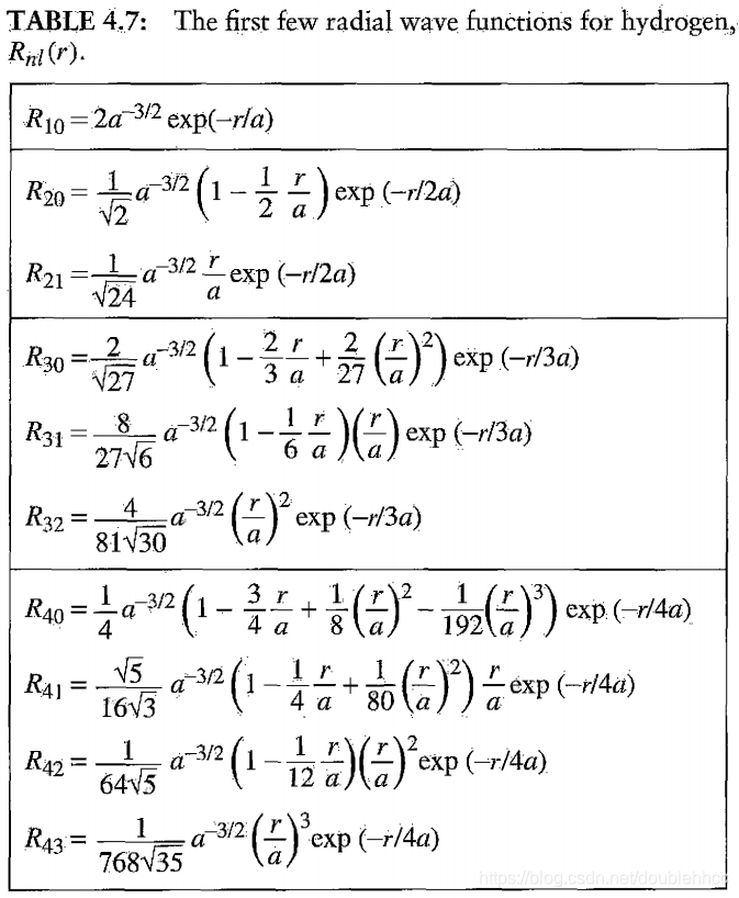
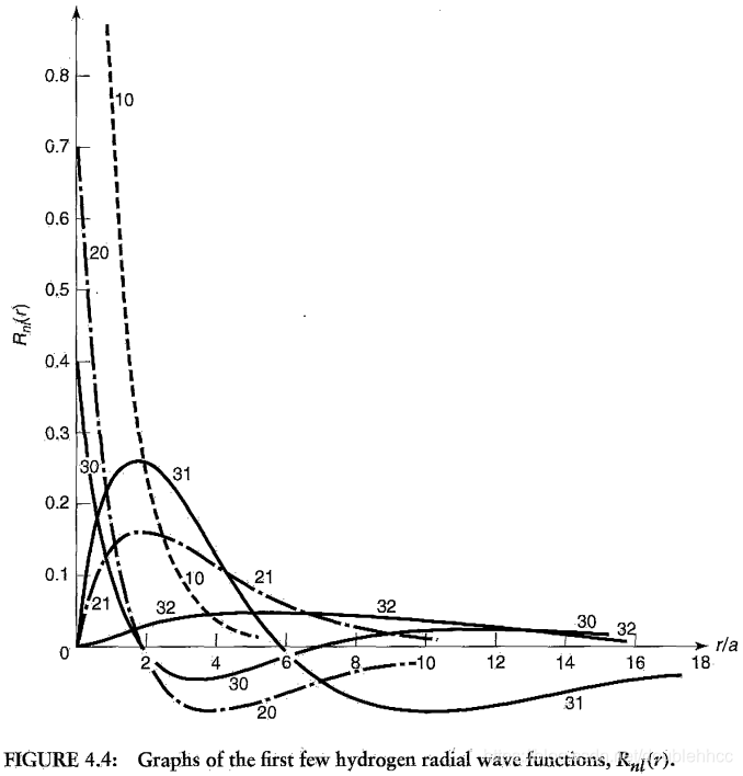
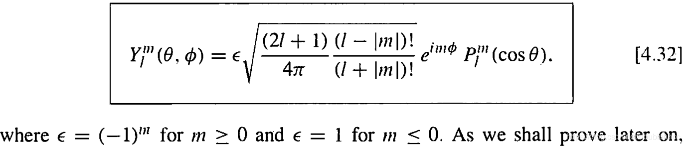
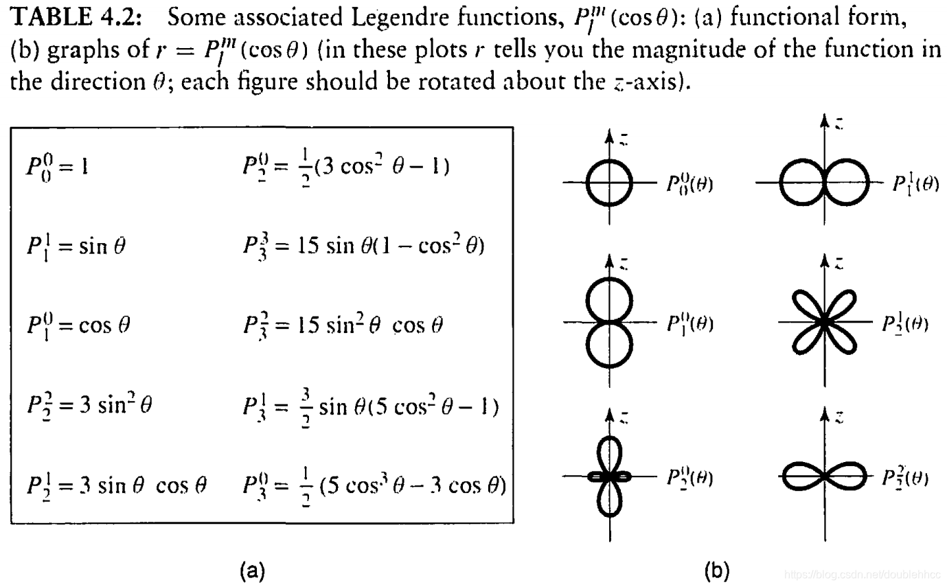
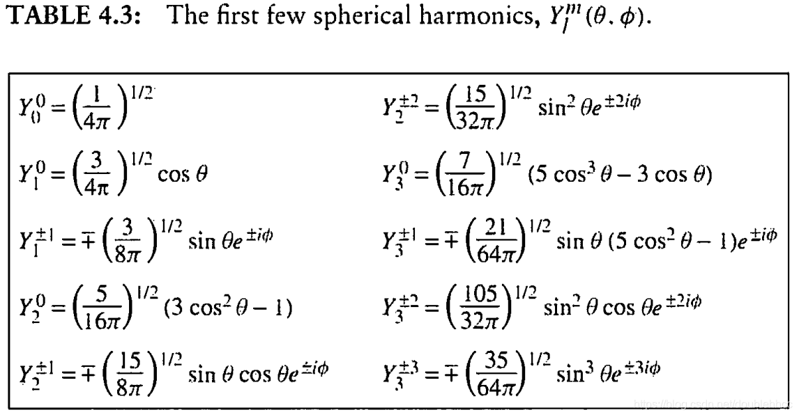
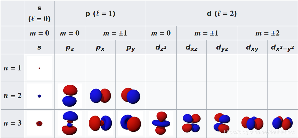
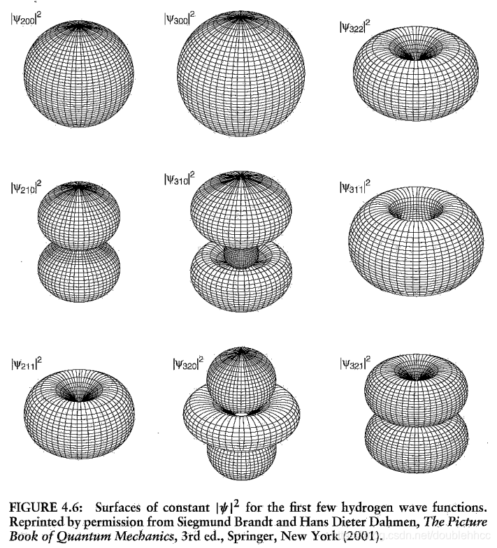
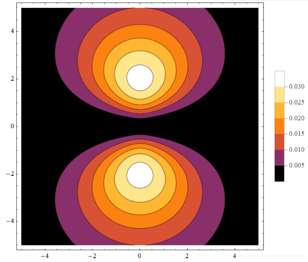
 本文通过Griffiths的量子力学书籍提供的资源,直观地展示了氢原子的波函数ψnlm(r,θ,ϕ),包括径向波函数Rnl(r)和球谐函数Ylm(θ,ϕ)。文章包含前几个径向波函数的表格和球谐函数的等高面图像,解释了px、py、pz轨道的形成,并提供了∣ψ∣2的等高面。此外,还探讨了如何利用奇偶性快速判断积分Ha,b′的非零项。"
20127615,1468723,Android Activity启动模式与Task、Process关系解析,"['Android开发', '任务栈', '回退栈', 'Activity管理', '应用架构']
本文通过Griffiths的量子力学书籍提供的资源,直观地展示了氢原子的波函数ψnlm(r,θ,ϕ),包括径向波函数Rnl(r)和球谐函数Ylm(θ,ϕ)。文章包含前几个径向波函数的表格和球谐函数的等高面图像,解释了px、py、pz轨道的形成,并提供了∣ψ∣2的等高面。此外,还探讨了如何利用奇偶性快速判断积分Ha,b′的非零项。"
20127615,1468723,Android Activity启动模式与Task、Process关系解析,"['Android开发', '任务栈', '回退栈', 'Activity管理', '应用架构']


 2524
2524


 到【灌水乐园】发言


