


本文来源公众号“天才程序员周弈帆”,仅用于学术分享,侵权删,干货满满。
原文链接:扩散模型(Diffusion Model)详解:直观理解、数学原理、PyTorch 实现
文章略长,分为天才程序员周弈帆 | 扩散模型(Diffusion Model)详解:直观理解、数学原理、PyTorch 实现(上)-优快云博客(上)和(下)两部分。
附录:代码复现
在这个项目中,我们要用PyTorch实现一个基于U-Net的DDPM,并在MNIST数据集(经典的手写数字数据集)上训练它。模型几分钟就能训练完,我们可以方便地做各种各样的实验。
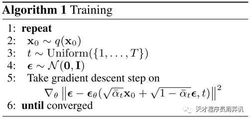
后续讲解只会给出代码片段,完整的代码请参见 https://github.com/SingleZombie/DL-Demos/tree/master/dldemos/ddpm 。git clone 仓库并安装后,可以直接运行目录里的main.py训练模型并采样。
获取数据集
PyTorch的torchvision提供了获取了MNIST的接口,我们只需要用下面的函数就可以生成MNIST的Dataset实例。参数中,root为数据集的下载路径,download为是否自动下载数据集。令download=True的话,第一次调用该函数时会自动下载数据集,而第二次之后就不用下载了,函数会读取存储在root里的数据。
mnist = torchvision.datasets.MNIST(root='./data/mnist', download=True)
我们可以用下面的代码来下载MNIST并输出该数据集的一些信息:
import torchvision
from torchvision.transforms import ToTensor
def download_dataset():
    mnist = torchvision.datasets.MNIST(root='./data/mnist', download=True)
    print('length of MNIST', len(mnist))
    id = 4
    img, label = mnist[id]
    print(img)
    print(label)

    # On computer with monitor
    # img.show()

    img.save('work_dirs/tmp.jpg')
    tensor = ToTensor()(img)
    print(tensor.shape)
    print(tensor.max())
    print(tensor.min())

if __name__ == '__main__':
    download_dataset()
执行这段代码,输出大致为:
length of MNIST 60000
<PIL.Image.Image image mode=L size=28x28 at 0x7FB3F09CCE50>
9
torch.Size([1, 28, 28])
tensor(1.)
tensor(0.)
第一行输出表明,MNIST数据集里有60000张图片。而从第二行和第三行输出中,我们发现每一项数据由图片和标签组成,图片是大小为28x28的PIL格式的图片,标签表明该图片是哪个数字。我们可以用torchvision里的ToTensor()把PIL图片转成PyTorch张量,进一步查看图片的信息。最后三行输出表明,每一张图片都是单通道图片(灰度图),颜色值的取值范围是0~1。
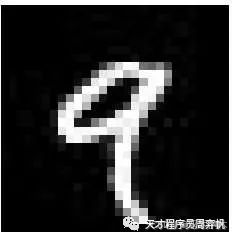
我们可以查看一下每张图片的样子。如果你是在用带显示器的电脑,可以去掉img.show那一行的注释,直接查看图片;如果你是在用服务器,可以去img.save的路径里查看图片。该图片的应该长这个样子:
我们可以用下面的代码预处理数据并创建DataLoader。由于DDPM会把图像和正态分布关联起来,我们更希望图像颜色值的取值范围是[-1, 1]。为此,我们可以对图像做一个线性变换,减0.5再乘2。
def get_dataloader(batch_size: int):
    transform = Compose([ToTensor(), Lambda(lambda x: (x - 0.5) * 2)])
    dataset = torchvision.datasets.MNIST(root='./data/mnist',
                                         transform=transform)
    return DataLoader(dataset, batch_size=batch_size, shuffle=True)
DDPM 类
在代码中,我们要实现一个DDPM类。它维护了扩散过程中的一些常量(比如),并且可以计算正向过程和反向过程的结果。
import torch

class DDPM():

    # n_steps 就是论文里的 T
    def __init__(self,
                 device,
                 n_steps: int,
                 min_beta: float = 0.0001,
                 max_beta: float = 0.02):
        betas = torch.linspace(min_beta, max_beta, n_steps).to(device)
        alphas = 1 - betas
        alpha_bars = torch.empty_like(alphas)
        product = 1
        for i, alpha in enumerate(alphas):
            product *= alpha
            alpha_bars[i] = product
        self.betas = betas
        self.n_steps = n_steps
        self.alphas = alphas
        self.alpha_bars = alpha_bars
部分实现会让 DDPM 继承
torch.nn.Module,但我认为这样不好。DDPM本身不是一个神经网络,它只是描述了前向过程和后向过程的一些计算。只有涉及可学习参数的神经网络类才应该继承torch.nn.Module。

def sample_forward(self, x, t, eps=None):
    alpha_bar = self.alpha_bars[t].reshape(-1, 1, 1, 1)
    if eps is None:
        eps = torch.randn_like(x)
    res = eps * torch.sqrt(1 - alpha_bar) + torch.sqrt(alpha_bar) * x
    return res
这里要解释一些PyTorch编程上的细节。这份代码中,self.alpha_bars是一个一维Tensor。而在并行训练中,我们一般会令t为一个形状为(batch_size, )的Tensor。PyTorch允许我们直接用self.alpha_bars[t]从self.alpha_bars里取出batch_size个数,就像用一个普通的整型索引来从数组中取出一个数一样。有些实现会用torch.gather从self.alpha_bars里取数,其作用是一样的。
我们可以随机从训练集取图片做测试,看看它们在前向过程中是怎么逐步变成噪声的。
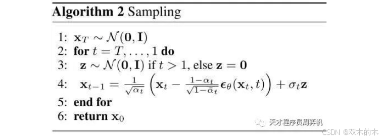
接下来实现反向过程。在反向过程中,DDPM会用神经网络预测每一轮去噪的均值,把xt复原回x0,以完成图像生成。反向过程即对应论文中的采样算法。
其实现如下:
def sample_backward(self, img_shape, net, device, simple_var=True):
    x = torch.randn(img_shape).to(device)
    net = net.to(device)
    for t in range(self.n_steps - 1, -1, -1):
        x = self.sample_backward_step(x, t, net, simple_var)
    return x

def sample_backward_step(self, x_t, t, net, simple_var=True):
    n = x_t.shape[0]
    t_tensor = torch.tensor([t] * n,
                            dtype=torch.long).to(x_t.device).unsqueeze(1)
    eps = net(x_t, t_tensor)

    if t == 0:
        noise = 0
    else:
        if simple_var:
            var = self.betas[t]
        else:
            var = (1 - self.alpha_bars[t - 1]) / (
                1 - self.alpha_bars[t]) * self.betas[t]
        noise = torch.randn_like(x_t)
        noise *= torch.sqrt(var)

    mean = (x_t -
            (1 - self.alphas[t]) / torch.sqrt(1 - self.alpha_bars[t]) *
            eps) / torch.sqrt(self.alphas[t])
    x_t = mean + noise

    return x_t
其中,sample_backward是用来给外部调用的方法,而sample_backward_step是执行一步反向过程的方法。
sample_backward会随机生成纯噪声x(对应xT),再令t从n_steps - 1到0,调用sample_backward_step。
def sample_backward(self, img_shape, net, device, simple_var=True):
    x = torch.randn(img_shape).to(device)
    net = net.to(device)
    for t in range(self.n_steps - 1, -1, -1):
        x = self.sample_backward_step(x, t, net, simple_var)
    return x
在sample_backward_step中,我们先准备好这一步的神经网络输出eps。为此,我们要把整型的t转换成一个格式正确的Tensor。考虑到输入里可能有多个batch,我们先获取batch size n,再根据它来生成t_tensor。
def sample_backward_step(self, x_t, t, net, simple_var=True):

    n = x_t.shape[0]
    t_tensor = torch.tensor([t] * n,
                            dtype=torch.long).to(x_t.device).unsqueeze(1)
    eps = net(x_t, t_tensor)
之后,我们来处理反向过程公式中的方差项。根据伪代码,我们仅在t非零的时候算方差项。方差项用到的方差有两种取值,效果差不多,我们用simple_var来控制选哪种取值方式。获取方差后,我们再随机采样一个噪声,根据公式,得到方差项。
if t == 0:
    noise = 0
else:
    if simple_var:
        var = self.betas[t]
    else:
        var = (1 - self.alpha_bars[t - 1]) / (
            1 - self.alpha_bars[t]) * self.betas[t]
    noise = torch.randn_like(x_t)
    noise *= torch.sqrt(var)
最后,我们把eps和方差项套入公式,得到这一步更新过后的图像x_t。
mean = (x_t -
        (1 - self.alphas[t]) / torch.sqrt(1 - self.alpha_bars[t]) *
        eps) / torch.sqrt(self.alphas[t])
x_t = mean + noise

return x_t
稍后完成了训练后,我们再来看反向过程的输出结果。
训练算法
接下来,我们先跳过神经网络的实现,直接完成论文里的训练算法。
再回顾一遍伪代码。首先,我们要随机选取训练图片x0,随机生成当前要训练的时刻t,以及随机生成一个生成的xt高斯噪声。之后,我们把xt和t输入进神经网络,尝试预测噪声。最后,我们以预测噪声和实际噪声的均方误差为损失函数做梯度下降。
为此,我们可以用下面的代码实现训练。
import torch
import torch.nn as nn
from dldemos.ddpm.dataset import get_dataloader, get_img_shape
from dldemos.ddpm.ddpm import DDPM
import cv2
import numpy as np
import einops

batch_size = 512
n_epochs = 100


def train(ddpm: DDPM, net, device, ckpt_path):
    # n_steps 就是公式里的 T
    # net 是某个继承自 torch.nn.Module 的神经网络
    n_steps = ddpm.n_steps
    dataloader = get_dataloader(batch_size)
    net = net.to(device)
    loss_fn = nn.MSELoss()
    optimizer = torch.optim.Adam(net.parameters(), 1e-3)

    for e in range(n_epochs):
        for x, _ in dataloader:
            current_batch_size = x.shape[0]
            x = x.to(device)
            t = torch.randint(0, n_steps, (current_batch_size, )).to(device)
            eps = torch.randn_like(x).to(device)
            x_t = ddpm.sample_forward(x, t, eps)
            eps_theta = net(x_t, t.reshape(current_batch_size, 1))
            loss = loss_fn(eps_theta, eps)
            optimizer.zero_grad()
            loss.backward()
            optimizer.step()
    torch.save(net.state_dict(), ckpt_path)
代码的主要逻辑都在循环里。首先是完成训练数据x0、t、噪声的采样。采样x0的工作可以交给PyTorch的DataLoader完成,每轮遍历得到的x就是训练数据。的采样可以用torch.randint函数随机从[0, n_steps - 1]取数。采样高斯噪声可以直接用torch.randn_like(x)生成一个和训练图片x形状一样的符合标准正态分布的图像。
for x, _ in dataloader:
    current_batch_size = x.shape[0]
    x = x.to(device)
    t = torch.randint(0, n_steps, (current_batch_size, )).to(device)
    eps = torch.randn_like(x).to(device)
之后计算xt并将其和t输入进神经网络net。计算xt的任务会由DDPM类的sample_forward方法完成,我们在上文已经实现了它。
x_t = ddpm.sample_forward(x, t, eps)
eps_theta = net(x_t, t.reshape(current_batch_size, 1))
得到了预测的噪声eps_theta,我们调用PyTorch的API,算均方误差并调用优化器即可。
loss_fn = nn.MSELoss()
optimizer = torch.optim.Adam(net.parameters(), 1e-3)

...
        loss = loss_fn(eps_theta, eps)
        optimizer.zero_grad()
        loss.backward()
        optimizer.step()
去噪神经网络
在DDPM中,理论上我们可以用任意一种神经网络架构。但由于DDPM任务十分接近图像去噪任务,而U-Net又是去噪任务中最常见的网络架构,因此绝大多数DDPM都会使用基于U-Net的神经网络。
我一直想训练一个尽可能简单的模型。经过多次实验,我发现DDPM的神经网络很难训练。哪怕是对于比较简单的MNIST数据集,结构差一点的网络(比如纯ResNet)都不太行,只有带了残差块和时序编码的U-Net才能较好地完成去噪。注意力模块倒是可以不用加上。
由于神经网络结构并不是DDPM学习的重点,我这里就不对U-Net的写法做解说,而是直接贴上代码了。代码中大部分内容都和普通的U-Net无异。唯一要注意的地方就是时序编码。去噪网络的输入除了图像外,还有一个时间戳t。我们要考虑怎么把t的信息和输入图像信息融合起来。大部分人的做法是对t进行Transformer中的位置编码,把该编码加到图像的每一处上。
import torch
import torch.nn as nn
import torch.nn.functional as F
from dldemos.ddpm.dataset import get_img_shape


class PositionalEncoding(nn.Module):

    def __init__(self, max_seq_len: int, d_model: int):
        super().__init__()

        # Assume d_model is an even number for convenience
        assert d_model % 2 == 0

        pe = torch.zeros(max_seq_len, d_model)
        i_seq = torch.linspace(0, max_seq_len - 1, max_seq_len)
        j_seq = torch.linspace(0, d_model - 2, d_model // 2)
        pos, two_i = torch.meshgrid(i_seq, j_seq)
        pe_2i = torch.sin(pos / 10000**(two_i / d_model))
        pe_2i_1 = torch.cos(pos / 10000**(two_i / d_model))
        pe = torch.stack((pe_2i, pe_2i_1), 2).reshape(max_seq_len, d_model)

        self.embedding = nn.Embedding(max_seq_len, d_model)
        self.embedding.weight.data = pe
        self.embedding.requires_grad_(False)

    def forward(self, t):
        return self.embedding(t)


class ResidualBlock(nn.Module):

    def __init__(self, in_c: int, out_c: int):
        super().__init__()
        self.conv1 = nn.Conv2d(in_c, out_c, 3, 1, 1)
        self.bn1 = nn.BatchNorm2d(out_c)
        self.actvation1 = nn.ReLU()
        self.conv2 = nn.Conv2d(out_c, out_c, 3, 1, 1)
        self.bn2 = nn.BatchNorm2d(out_c)
        self.actvation2 = nn.ReLU()
        if in_c != out_c:
            self.shortcut = nn.Sequential(nn.Conv2d(in_c, out_c, 1),
                                          nn.BatchNorm2d(out_c))
        else:
            self.shortcut = nn.Identity()

    def forward(self, input):
        x = self.conv1(input)
        x = self.bn1(x)
        x = self.actvation1(x)
        x = self.conv2(x)
        x = self.bn2(x)
        x += self.shortcut(input)
        x = self.actvation2(x)
        return x


class ConvNet(nn.Module):

    def __init__(self,
                 n_steps,
                 intermediate_channels=[10, 20, 40],
                 pe_dim=10,
                 insert_t_to_all_layers=False):
        super().__init__()
        C, H, W = get_img_shape()  # 1, 28, 28
        self.pe = PositionalEncoding(n_steps, pe_dim)

        self.pe_linears = nn.ModuleList()
        self.all_t = insert_t_to_all_layers
        if not insert_t_to_all_layers:
            self.pe_linears.append(nn.Linear(pe_dim, C))

        self.residual_blocks = nn.ModuleList()
        prev_channel = C
        for channel in intermediate_channels:
            self.residual_blocks.append(ResidualBlock(prev_channel, channel))
            if insert_t_to_all_layers:
                self.pe_linears.append(nn.Linear(pe_dim, prev_channel))
            else:
                self.pe_linears.append(None)
            prev_channel = channel
        self.output_layer = nn.Conv2d(prev_channel, C, 3, 1, 1)

    def forward(self, x, t):
        n = t.shape[0]
        t = self.pe(t)
        for m_x, m_t in zip(self.residual_blocks, self.pe_linears):
            if m_t is not None:
                pe = m_t(t).reshape(n, -1, 1, 1)
                x = x + pe
            x = m_x(x)
        x = self.output_layer(x)
        return x


class UnetBlock(nn.Module):

    def __init__(self, shape, in_c, out_c, residual=False):
        super().__init__()
        self.ln = nn.LayerNorm(shape)
        self.conv1 = nn.Conv2d(in_c, out_c, 3, 1, 1)
        self.conv2 = nn.Conv2d(out_c, out_c, 3, 1, 1)
        self.activation = nn.ReLU()
        self.residual = residual
        if residual:
            if in_c == out_c:
                self.residual_conv = nn.Identity()
            else:
                self.residual_conv = nn.Conv2d(in_c, out_c, 1)

    def forward(self, x):
        out = self.ln(x)
        out = self.conv1(out)
        out = self.activation(out)
        out = self.conv2(out)
        if self.residual:
            out += self.residual_conv(x)
        out = self.activation(out)
        return out


class UNet(nn.Module):

    def __init__(self,
                 n_steps,
                 channels=[10, 20, 40, 80],
                 pe_dim=10,
                 residual=False) -> None:
        super().__init__()
        C, H, W = get_img_shape()
        layers = len(channels)
        Hs = [H]
        Ws = [W]
        cH = H
        cW = W
        for _ in range(layers - 1):
            cH //= 2
            cW //= 2
            Hs.append(cH)
            Ws.append(cW)

        self.pe = PositionalEncoding(n_steps, pe_dim)

        self.encoders = nn.ModuleList()
        self.decoders = nn.ModuleList()
        self.pe_linears_en = nn.ModuleList()
        self.pe_linears_de = nn.ModuleList()
        self.downs = nn.ModuleList()
        self.ups = nn.ModuleList()
        prev_channel = C
        for channel, cH, cW in zip(channels[0:-1], Hs[0:-1], Ws[0:-1]):
            self.pe_linears_en.append(
                nn.Sequential(nn.Linear(pe_dim, prev_channel), nn.ReLU(),
                              nn.Linear(prev_channel, prev_channel)))
            self.encoders.append(
                nn.Sequential(
                    UnetBlock((prev_channel, cH, cW),
                              prev_channel,
                              channel,
                              residual=residual),
                    UnetBlock((channel, cH, cW),
                              channel,
                              channel,
                              residual=residual)))
            self.downs.append(nn.Conv2d(channel, channel, 2, 2))
            prev_channel = channel

        self.pe_mid = nn.Linear(pe_dim, prev_channel)
        channel = channels[-1]
        self.mid = nn.Sequential(
            UnetBlock((prev_channel, Hs[-1], Ws[-1]),
                      prev_channel,
                      channel,
                      residual=residual),
            UnetBlock((channel, Hs[-1], Ws[-1]),
                      channel,
                      channel,
                      residual=residual),
        )
        prev_channel = channel
        for channel, cH, cW in zip(channels[-2::-1], Hs[-2::-1], Ws[-2::-1]):
            self.pe_linears_de.append(nn.Linear(pe_dim, prev_channel))
            self.ups.append(nn.ConvTranspose2d(prev_channel, channel, 2, 2))
            self.decoders.append(
                nn.Sequential(
                    UnetBlock((channel * 2, cH, cW),
                              channel * 2,
                              channel,
                              residual=residual),
                    UnetBlock((channel, cH, cW),
                              channel,
                              channel,
                              residual=residual)))

            prev_channel = channel

        self.conv_out = nn.Conv2d(prev_channel, C, 3, 1, 1)

    def forward(self, x, t):
        n = t.shape[0]
        t = self.pe(t)
        encoder_outs = []
        for pe_linear, encoder, down in zip(self.pe_linears_en, self.encoders,
                                            self.downs):
            pe = pe_linear(t).reshape(n, -1, 1, 1)
            x = encoder(x + pe)
            encoder_outs.append(x)
            x = down(x)
        pe = self.pe_mid(t).reshape(n, -1, 1, 1)
        x = self.mid(x + pe)
        for pe_linear, decoder, up, encoder_out in zip(self.pe_linears_de,
                                                       self.decoders, self.ups,
                                                       encoder_outs[::-1]):
            pe = pe_linear(t).reshape(n, -1, 1, 1)
            x = up(x)

            pad_x = encoder_out.shape[2] - x.shape[2]
            pad_y = encoder_out.shape[3] - x.shape[3]
            x = F.pad(x, (pad_x // 2, pad_x - pad_x // 2, pad_y // 2,
                          pad_y - pad_y // 2))
            x = torch.cat((encoder_out, x), dim=1)
            x = decoder(x + pe)
        x = self.conv_out(x)
        return x


convnet_small_cfg = {
    'type': 'ConvNet',
    'intermediate_channels': [10, 20],
    'pe_dim': 128
}

convnet_medium_cfg = {
    'type': 'ConvNet',
    'intermediate_channels': [10, 10, 20, 20, 40, 40, 80, 80],
    'pe_dim': 256,
    'insert_t_to_all_layers': True
}
convnet_big_cfg = {
    'type': 'ConvNet',
    'intermediate_channels': [20, 20, 40, 40, 80, 80, 160, 160],
    'pe_dim': 256,
    'insert_t_to_all_layers': True
}

unet_1_cfg = {'type': 'UNet', 'channels': [10, 20, 40, 80], 'pe_dim': 128}
unet_res_cfg = {
    'type': 'UNet',
    'channels': [10, 20, 40, 80],
    'pe_dim': 128,
    'residual': True
}


def build_network(config: dict, n_steps):
    network_type = config.pop('type')
    if network_type == 'ConvNet':
        network_cls = ConvNet
    elif network_type == 'UNet':
        network_cls = UNet

    network = network_cls(n_steps, **config)
    return network
实验结果与采样
把之前的所有代码综合一下,我们以带残差块的U-Net为去噪网络,执行训练。
if __name__ == '__main__':
    n_steps = 1000
    config_id = 4
    device = 'cuda'
    model_path = 'dldemos/ddpm/model_unet_res.pth'

    config = unet_res_cfg
    net = build_network(config, n_steps)
    ddpm = DDPM(device, n_steps)

    train(ddpm, net, device=device, ckpt_path=model_path)
按照默认训练配置,在3090上花5分钟不到,训练30~40个epoch即可让网络基本收敛。最终收敛时loss在0.023~0.024左右。
batch size: 512
epoch 0 loss: 0.23103461712201437 elapsed 7.01s
epoch 1 loss: 0.0627968365987142 elapsed 13.66s
epoch 2 loss: 0.04828845852613449 elapsed 20.25s
epoch 3 loss: 0.04148937337398529 elapsed 26.80s
epoch 4 loss: 0.03801360730528831 elapsed 33.37s
epoch 5 loss: 0.03604260584712028 elapsed 39.96s
epoch 6 loss: 0.03357676289876302 elapsed 46.57s
epoch 7 loss: 0.0335664684087038 elapsed 53.15s
...
epoch 30 loss: 0.026149748386939366 elapsed 204.64s
epoch 31 loss: 0.025854381563266117 elapsed 211.24s
epoch 32 loss: 0.02589433005253474 elapsed 217.84s
epoch 33 loss: 0.026276464049021404 elapsed 224.41s
...
epoch 96 loss: 0.023299352884292603 elapsed 640.25s
epoch 97 loss: 0.023460942271351815 elapsed 646.90s
epoch 98 loss: 0.023584651704629263 elapsed 653.54s
epoch 99 loss: 0.02364126600921154 elapsed 660.22s
训练这个网络时,并没有特别好的测试指标,我们只能通过观察采样图像来评价网络的表现。我们可以用下面的代码调用DDPM的反向传播方法,生成多幅图像并保存下来。
def sample_imgs(ddpm,
                net,
                output_path,
                n_sample=81,
                device='cuda',
                simple_var=True):
    net = net.to(device)
    net = net.eval()
    with torch.no_grad():
        shape = (n_sample, *get_img_shape())  # 1, 3, 28, 28
        imgs = ddpm.sample_backward(shape,
                                    net,
                                    device=device,
                                    simple_var=simple_var).detach().cpu()
        imgs = (imgs + 1) / 2 * 255
        imgs = imgs.clamp(0, 255)
        imgs = einops.rearrange(imgs,
                                '(b1 b2) c h w -> (b1 h) (b2 w) c',
                                b1=int(n_sample**0.5))

        imgs = imgs.numpy().astype(np.uint8)

        cv2.imwrite(output_path, imgs)
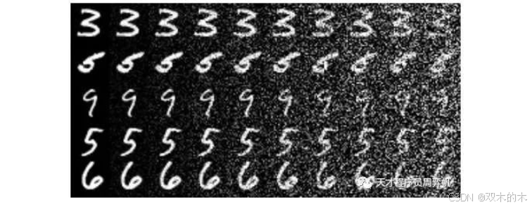
一切顺利的话,我们可以得到一些不错的生成结果。下图是我得到的一些生成图片:
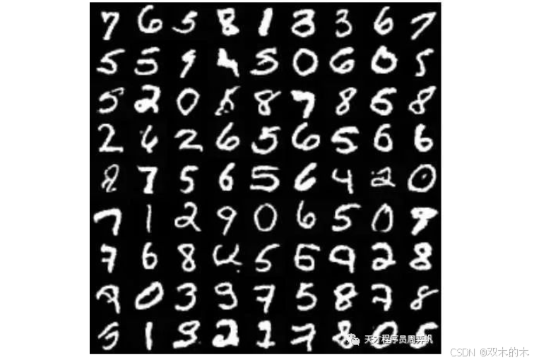
大部分生成的图片都对应一个阿拉伯数字,它们和训练集MNIST里的图片非常接近。这算是一个不错的生成结果。
如果神经网络的拟合能力较弱,生成结果就会差很多。下图是我训练一个简单的ResNet后得到的采样结果:
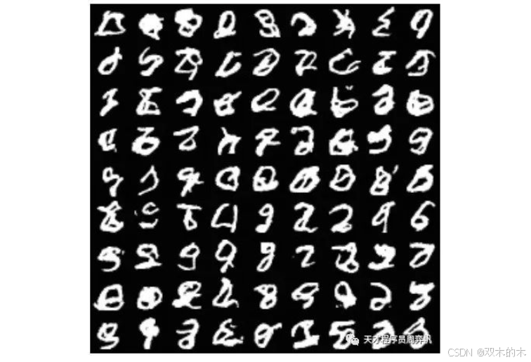
可以看出,每幅图片都很乱,基本对应不上一个数字。这就是一个较差的训练结果。
如果网络再差一点,可能会生成纯黑或者纯白的图片。这是因为网络的预测结果不准,在反向过程中,图像的均值不断偏移,偏移到远大于1或者远小于-1的值了。
总结一下,在复现DDPM时,最主要是要学习DDPM论文的两个算法,即训练算法和采样算法。两个算法很简单,可以轻松地把它们翻译成代码。而为了成功完成复现,还需要花一点心思在编写U-Net上,尤其是注意处理时间戳的部分。
THE END !
文章结束,感谢阅读。您的点赞,收藏,评论是我继续更新的动力。大家有推荐的公众号可以评论区留言,共同学习,一起进步。


 1261
1261

 被折叠的 条评论
为什么被折叠?
被折叠的 条评论
为什么被折叠?
 到【灌水乐园】发言


