

李航统计学习--感知机算法实现(python)

感知机学习总结及例题(附代码及手算过程) 感知机是一种二类分类的线性分类模型,其输入为实例的特征向量,输出为实例的类别,+1代表正类,-1代表负类,是神经网络和支持向量机的基础。 例如一个典型的二分类问题:银行卡申请问题,对于顾客,决定是否给予信用卡 对于一个顾客的信息(年龄、薪资、当前债务等等),我们可以用一个向量表示。然后每个信息条目(维度)均对是否给他信用卡有着正面或者负面的影响,决定我们是否给他信用卡。我们把这些维度加权叠加计算出来,结果若大于某个阈值就给,否则就不给。 设X=(x1,x2,...,xd)X = (x_1,x_2,...,x 阅读详情
AI摘要

本文介绍了感知机模型及其学习算法,包括损失函数的定义及随机梯度下降法的应用,并通过鸢尾花数据集实现了手动编写感知机算法及使用sklearn库进行二分类任务。

感知机

1.感知机是根据输入实例的特征向量xxx对其进行二类分类的线性分类模型:

f(x)=sign⁡(w⋅x+b)f(x)=\operatorname{sign}(w \cdot x+b)f(x)=sign(w⋅x+b)

感知机模型对应于输入空间(特征空间)中的分离超平面w⋅x+b=0w \cdot x+b=0w⋅x+b=0。

2.感知机学习的策略是极小化损失函数:

min⁡w,bL(w,b)=−∑xi∈Myi(w⋅xi+b)\min _{w, b} L(w, b)=-\sum_{x_{i} \in M} y_{i}\left(w \cdot x_{i}+b\right)w,bmin​L(w,b)=−xi​∈M∑​yi​(w⋅xi​+b)

损失函数对应于误分类点到分离超平面的总距离。

3.感知机学习算法是基于随机梯度下降法的对损失函数的最优化算法,有原始形式和对偶形式。算法简单且易于实现。原始形式中,首先任意选取一个超平面,然后用梯度下降法不断极小化目标函数。在这个过程中一次随机选取一个误分类点使其梯度下降。

4.当训练数据集线性可分时,感知机学习算法是收敛的。感知机算法在训练数据集上的误分类次数kkk满足不等式:

k⩽(Rγ)2k \leqslant\left(\frac{R}{\gamma}\right)^{2}k⩽(γR​)2

当训练数据集线性可分时,感知机学习算法存在无穷多个解,其解由于不同的初值或不同的迭代顺序而可能有所不同。


感知机模型

f(x)=sign(w⋅x+b)f(x) = sign(w\cdot x + b)f(x)=sign(w⋅x+b)

sign⁡(x)={+1,x⩾0−1,x<0\operatorname{sign}(x)=\left\{\begin{array}{ll}{+1,} & {x \geqslant 0} \\ {-1,} & {x<0}\end{array}\right.sign(x)={+1,−1,​x⩾0x<0​

给定训练集:

T={(x1,y1),(x2,y2),⋯ ,(xN,yN)}T=\left\{\left(x_{1}, y_{1}\right),\left(x_{2}, y_{2}\right), \cdots,\left(x_{N}, y_{N}\right)\right\}T={(x1​,y1​),(x2​,y2​),⋯,(xN​,yN​)}

定义感知机的损失函数

L(w,b)=−∑xi∈Myi(w⋅xi+b)L(w, b)=-\sum_{x_{i} \in M} y_{i}\left(w \cdot x_{i}+b\right)L(w,b)=−∑xi​∈M​yi​(w⋅xi​+b)


算法

随即梯度下降法 Stochastic Gradient Descent

随机抽取一个误分类点使其梯度下降。
若 yi(w⋅xi+b)⩽0y_{i}\left(w \cdot x_{i}+b\right)\leqslant 0yi​(w⋅xi​+b)⩽0
则判断为误分类点,然后进行w和b的更新:

w=w+ηyixiw = w + \eta y_{i}x_{i}w=w+ηyi​xi​

b=b+ηyib = b + \eta y_{i}b=b+ηyi​

当实例点被误分类,即位于分离超平面的错误侧,则调整www, bbb的值,使分离超平面向该无分类点的一侧移动,直至误分类点被正确分类,其中η\etaη为学习率

实现1将手动实现感知机算法,数据集则采用sklearn中鸢尾花数据集。

数据集介绍:iris数据集由Fisher在1936年整理,包含4个特征(Sepal.Length(花萼长度)、Sepal.Width(花萼宽度)、Petal.Length(花瓣长度)、Petal.Width(花瓣宽度)),特征值都为正浮点数,单位为厘米。目标值为鸢尾花的分类(Iris Setosa(山鸢尾)、Iris Versicolour(杂色鸢尾),Iris Virginica(维吉尼亚鸢尾))。
为了实现感知机算法,本文拿出iris数据集中两个分类的数据和[sepal length,sepal width]作为特征,去识别出花的类型。

实现1:

# @Author: coderdz
# @File: Perceptron.py
# @Site: github.com/dingzhen7186
# @Ended Time : 2020/9/21

import numpy as np
import matplotlib.pyplot as plt
import pandas as pd
from sklearn.datasets import load_iris

class Perceptron():
	def __init__(self):
		 # w初始化为全1数组
		self.w = np.ones(len(data[0]) - 1, dtype = np.float32)
		self.b = 0
		self.rate = 0.5 # 初始化学习率
	
	# 感知机训练, 找出最合适的w, b
	def fit(self, x_train, y_train):
		while True:
			flag = True # 标记是否存在误分类数据
			for i in range(len(x_train)): # 遍历训练数据
				xi = x_train[i]
				yi = y_train[i]
				 # 判断 yi * (wx + b) <= 0
				if yi * (np.inner(self.w, xi) + self.b) <= 0:
					flag = False # 找到误分类数据, flag标记为False
					 # 更新w, b值
					self.w += self.rate * np.dot(xi, yi)
					self.b += self.rate * yi
			if flag:
				break
		 # 输出w = ? , b = ?
		print('w = ' + str(self.w) + ', b = ' + str(self.b))

	# 图形显示结果
	def show(self, data):
		x_ = np.linspace(4, 7, 10)
		y_ = -(self.w[0] * x_ + self.b) / self.w[1]
		 # 画出这条直线
		plt.plot(x_, y_)
		 # 画出数据集的散点图
		plt.plot(data[:50, 0], data[:50, 1], 'bo', c = 'blue', label = '0')
		plt.plot(data[50:100, 0], data[50:100, 1], 'bo', c = 'orange', label = '1')
		plt.xlabel('sepal length')
		plt.ylabel('sepal width')
		plt.legend()
		plt.show()

iris = load_iris()
# 通过DataFrmae对象获取iris数据集对象, 列名为该数据集样本的特征名
df = pd.DataFrame(iris.data, columns = iris.feature_names)
# 增加label列为它们的分类标签
df['label'] = iris.target
df.columns = ['sepal length', 'sepal width', 'petal length', 'petal width', 'label']
#print(df.label.value_counts()) 不同标签的样本数量
# 2:50 1:50 0:50

# 画出散点图查看特征点的分布
plt.scatter(df[:50]['sepal length'].values, df[:50]['sepal width'].values, label='0')
plt.scatter(df[50:100]['sepal length'].values, df[50:100]['sepal width'].values, label='1')
plt.xlabel('sepal length')
plt.ylabel('sepal width')
plt.legend()
plt.show()

# 选择数据集
data = np.array(df.iloc[:100, [0, 1, -1]])
# 数据集划分
x, y = data[:, :-1], data[:, -1]
# 将y数据集值变为1和-1
y = np.array([1 if i == 1 else -1 for i in y])

# 开始训练
p = Perceptron()
p.fit(x, y)
p.show(data)

输出如下:

w = [ 39.85006  -50.400837], b = -63.5
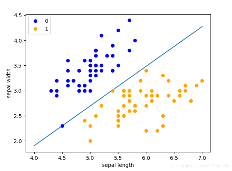
在这里插入图片描述


实现2将采用sklearn中已经实现好了的Perceptron感知机,然后调用相关方法实现二分类。

实现2:

# @Author: coderdz
# @File: Perceptron.py
# @Site: github.com/dingzhen7186
# @Ended Time : 2020/9/21

import sklearn
from sklearn.linear_model import Perceptron
from sklearn.datasets import load_iris
import pandas as pd
import matplotlib.pyplot as plt
import numpy as np

# 数据预处理
iris = load_iris()
df = pd.DataFrame(iris.data, columns = iris.feature_names)
df['label'] = iris.target
df.columns = ['sepal length', 'sepal width', 'petal length', 'petal width', 'label']
data = np.array(df.iloc[:100, [0, 1, -1]])
x, y = data[:, :-1], data[:, -1]
y = np.array([1 if i == 1 else -1 for i in y])

# 模型训练
clf = Perceptron(fit_intercept = True, max_iter = 1000, tol = None, shuffle = True)
clf.fit(x, y)
# 输出参数w, b
print('w = ' + str(clf.coef_) + ', b = ' + str(clf.intercept_))

# 画出图形
plt.figure(figsize = (10, 10)) #设置画布大小
plt.rcParams['font.sans-serif'] = ['SimHei']
plt.rcParams['axes.unicode_minus'] = False
plt.title('鸢尾花线性数据示例')

# 画出散点图, iris-setosa:山鸢尾, iris-versicolour: 杂色鸢尾
plt.scatter(data[:50, 0], data[:50, 1], c = 'b', label = 'iris-setosa')
plt.scatter(data[50:100, 0], data[50:100, 1], c = 'orange', label = 'iris-versicolor')

# 画出感知机的线
x_ = np.arange(4, 8)
y_ = -(clf.coef_[0][0]*x_ + clf.intercept_) / clf.coef_[0][1]
plt.plot(x_, y_)

plt.legend() # 显示图例
plt.grid(False) # 不显示网络
plt.xlabel('sepal length')
plt.ylabel('sepal width')
plt.show()

输出如下:

w = [[ 66.1 -83.3]], b = [-106.]
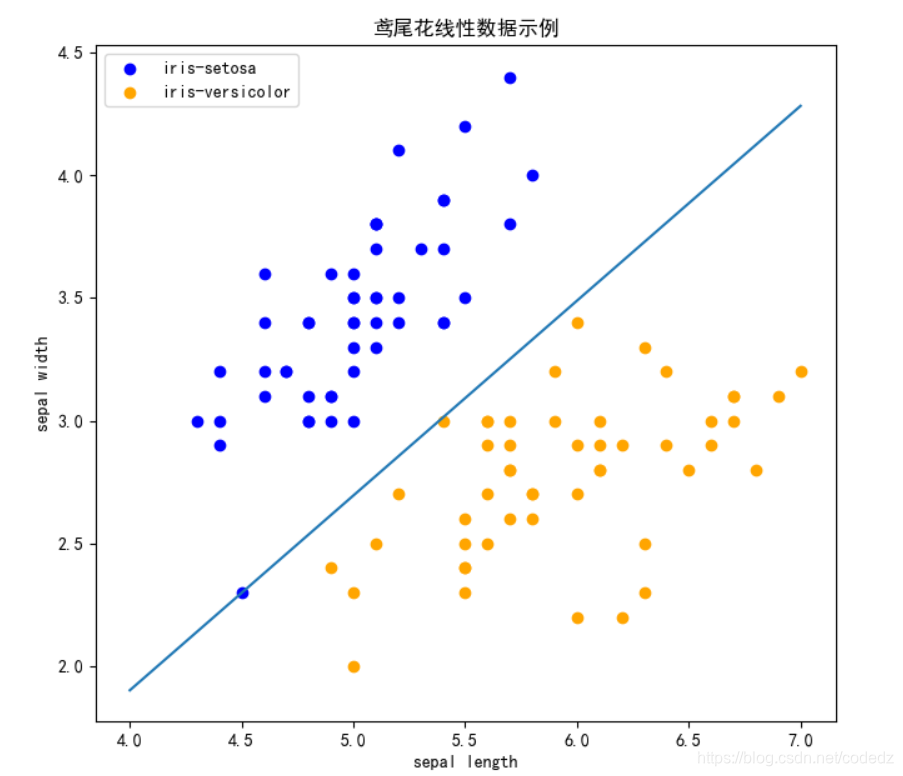
在这里插入图片描述
我的导师李胜开组会说了一句话,我觉得说的很好,“前途是光明的,道路是曲折的”,大家一起加油吧!

李航《统计学习方法》第2版 第2章课后习题答案 习题2.1 题目:Minsky与Papert指出:感知机因为是线性模型,所以不能表示复杂的函数,如异或(XOR),验证感知机为什么不能表示异或。 习题2.2 题目:模仿例题2.1,构建从训练数据集求解感知机模型的例子。 解:这里用python代码分别实现一下感知机学习算法的原始形式与对偶形式 原始形式: """ 感知机(原始形式):实现书本P40页 例题2.1 """ import numpy as np import matplotlib.pyplot as plt class MyPerceptr 阅读详情

相关推荐

YOLOv8中Bottleneck模块的残差连接机制解析

本文深入解析了YOLOv8目标检测模型中Bottleneck模块的核心设计,重点阐述了其残差连接机制。该机制通过构建一条信息“捷径”,有效缓解了深层网络中的梯度消失问题,稳定了训练过程,并提升了特征提取效率。文章结合代码详细拆解了模块结构,并探讨了其在YOLOv8骨干网络与检测头中的关键作用及参数调优思路。

weixin_29061821的博客 253

感知机算法之Python代码实现

感知机算法之Python代码实现

water lover的博客 5871

FairyGUI编辑器自定义菜单扩展插件

本文涉及到的软件有:FairyGUI,VSCode代码环境涉及到了:LuaVSCode插件:EmmyLua在编写FairyGUI编辑器菜单前,了解一下FairyGUIEditor的API会有效的帮助我们解决很多问题。FairyGUI的扩展是通过编辑器自带的插件功能实现的,插件中我使用的是lua环境模板。导入编辑器的LuaAPI,文件可以在FairyGUI-Editor源码的插件目录中找到。接下来将通过功能来说明对应的API作用。

Aili_Xiao的博客 4496

感知机算法的python实现

本文介绍了利用pthon实现二维空间下的感知机算法

ZhuhaoNan134的博客 1796

Android逆向实战:用Xposed Hook微信消息发送(附完整代码)

本文提供了一份Android逆向实战指南,详细讲解如何使用Xposed框架Hook微信消息发送功能。内容涵盖环境搭建、逆向分析定位关键方法、编写Hook模块代码以及调试部署的全过程,并附有完整代码示例,帮助开发者深入理解Android应用底层交互与Hook技术。

weixin_29196315的博客 1117

DDR4协议规范之(一)DDR4结构和寻址

DDR4 SDRAM结构和寻址DDR4 SDRAM的封装和寻址新的改变功能快捷键合理的创建标题,有助于目录的生成如何改变文本的样式插入链接与图片如何插入一段漂亮的代码片生成一个适合你的列表创建一个表格设定内容居中、居左、居右SmartyPants创建一个自定义列表如何创建一个注脚注释也是必不可少的KaTeX数学公式新的甘特图功能,丰富你的文章UML 图表FLowchart流程图导出与导入导出导入 DDR4 SDRAM的封装和寻址 你好! 这是你第一次使用 Markdown编辑器 所展示的欢迎页。如果你想学习

YJFeiii的博客 3万+

感知机算法python实现

感知机(perceptron)是二分类的线性分类模型,其中输入是实例的特征向量,输出是类别,类别取+1和-1二值。感知机的目标是求出一个超平面将训练数据进行线性划分。 下面基于鸢尾花数据进行实现感知机算法。 简单介绍下鸢尾花数据:iris数据集的中文名是安德森鸢尾花卉数据集,英文全称是Anderson’s Iris data set。iris数据集是一个150行5列的二维表。具体来说是150个样本,每个样本是数据集中的每行数据,每个样本有4个特征(前4列),1个标签(第五列)。4个特征分别是花萼长度、花

sendiae的博客 3445

【ESP32设备通信】-LoRaWAN网关

在物联网 (IoT) 时代,连接设备和收集数据变得比以往任何时候都更加容易和重要。 LoRaWAN(远程广域网)技术已成为远程、低功耗物联网通信的强大解决方案。 在本教程中,我们将使用 ESp32 构建 LoRaWAN 网关电路,并使用 ESP32 和 BME280 传感器构建传感器节点电路。 对于这两个电路,我们将使用基于 SX1278 (Ra-02) LoRa 模块在设备之间进行无线通信。 我们还将向您展示如何将传感器数据传输到流行的物联网平台 ThingSpeak。

视觉与物联智能 1580

用Python实现感知器学习算法

感知器原理+用Python实现一个感知器

qq_41697157的博客 851

【YOLOv8科研级优化】基于YOLOv9的GELAN模块重构C2f结构,实现精度与效率的同步提升

打开确保模型解析器能识别GELANBlock模块。通过将YOLOv9的GELAN模块集成到YOLOv8的C2f模块中,我们实现了一个“强特征表达+高效计算”的目标检测模型。这个改进不仅在工程上能提升复杂场景下的检测效果,更在科研上提供了“多分支特征融合”的创新思路——这种思路可以延伸到其他检测网络(如Faster R-CNN、SSD)的改进中,帮你在论文中打造独特的研究点。

know_F0727的博客 201

如何离线环境下安装Dify插件 (可提供远程指导协助)

离线环境下安装Dify插件

litlit023的专栏 8100

Python实现感知机算法——李航《统计学习方法》

接下来一学期选了门《机器学习》的课程,所以打算把相关的作业也发上来! 一: 请说明感知机为何不能解决异或问题。 答:我们知道感知机属于线性模型,由于其无法找到一个线性模型对异或问题进行划分,所以其不能解决异或问题。具体解释如下: 首先我们知道感知机的数学表达式就是: f(x)=sign(wx+b) 其中sign是符号函数,w和b都是感知机参数,x表示实例的特征向量,而y=f(x)就是实例的类别。以...

qq_37335890的博客 1818

笔试题-2023-紫光展锐-数字芯片设计【纯净题目版】

笔试题-2023-紫光展锐-数字芯片设计【纯净题目版】

w0shishabi的博客 2923

感知机学习算法代码简单实现

感知机算是一个比较简单的算法了,原理网上有很多,有原始形式和对偶形式两种,感觉自己比较菜,觉得慢慢从头把新版的李航统计学习方法自己实现一遍,明年就要实习了,慌得一批,这里仅把算法描述和原始形式的简单形式用python实现以下,供自己日后复习: # -*- coding:utf-8 -*- import numpy as np # 感知机学习算法demo data = np.array([[3,...

熊伟 910

大中型超市收银系统(可直接运行)

光步前台收银系统系统功能:商品销售、商品退货、挂单、收银员权限、会员销售、单品取消、整单取消、商品查询、脱机销售、脱机数据上传,基本资料下载,开钱箱、小票打印、收款结算,支持多币种付款方式(现金、储值卡、礼券、微信等),支持多种促销。运行环境:.net 4.0登陆信息用户名:1001 密码:123456内置商品信息,商品编码可输入00001000 - 00010000,测试效果相关功能键F5 结算 F9挂单 F11商品查询 F8退货 Insert单品取消 Del整单取消 F12开钱箱F2 会员 Ctrl+Z退出系统 Home 锁屏 相关源码待公开

汉书HE8,好用的汇编代码编写工具

汉书HE8,好用的汇编代码编写工具早期编写汇编代码所用功能强大

[转]统计学习方法—chapter2—感知机算法实现

描述:李航《统计学习方法》第二章感知机算法实现(Python) 原始形式: 1 # _*_ encoding:utf-8 _*_ 2 3 import numpy as np 4 import matplotlib.pyplot as plt 5 6 7 def createdata(): 8 """创建数据集和相应类标记""" 9 ...

weixin_30371469的博客 156

蓝牙模块HM-10手册

蓝牙模块HM-10手册,该手册对蓝牙模块HM-10进行了详细的介绍和使用方法以及一些AT指令。

AiPy中的统计学习方法:李航教授经典教材实战指南

想要掌握机器学习核心算法但不知从何入手?AiPy项目为你提供了李航教授《统计学习方法》的完整实战代码库!这个开源项目将经典机器学习理论与Python代码实现完美结合,是新手入门和普通用户学习统计学习方法的最佳选择。 ## 📚 为什么选择AiPy学习统计学习方法? AiPy项目汇集了Python机器学习、深度学习算法的学习资源,其中最核心的部分就是**统计学习方法实战代码库**。这个资源库包含

gitblog_00168的博客 230

深度学习工具包 DeepLearningToolbox

深度学习工具包Deprecation notice.-----This toolbox is outdated and no longer maintained.There are much better tools available for deep learning than this toolbox, e.g. [Theano](http://deeplearning.net/software/theano/), [torch](http://torch.ch/) or [tensorflow](http://www.tensorflow.org/)I would suggest you use one of the tools mentioned above rather than use this toolbox.Best, Rasmus.DeepLearnToolbox================A Matlab toolbox for Deep Learning.Deep Learning is a new subfield of machine learning that focuses on learning deep hierarchical models of data.It is inspired by the human brain's apparent deep (layered, hierarchical) architecture.A good overview of the theory of Deep Learning theory is[Learning Deep Architectures for AI](http://www.iro.umontreal.ca/~bengioy/papers/ftml_book.pdf)For a more informal introduction, see the following videos by Geoffrey Hinton and Andrew Ng.* [The Next Generation of Neural Networks](http://www.youtube.com/watch?v=AyzOUbkUf3M) (Hinton, 2007)* [Recent Developments in Deep Learning](http://www.youtube.com/watch?v=VdIURAu1-aU) (Hinton, 2010)* [Unsupervised Feature Learning and Deep Learning](http://www.youtube.com/watch?v=ZmNOAtZIgIk) (Ng, 2011)If you use this toolbox in your research please cite [Prediction as a candidate for learning deep hierarchical models of data](http://www2.imm.dtu.dk/pubdb/views/publication_details.php?id=6284)```@MASTERSTHESIS\{IMM2012-06284, author = "R. B. Palm", title = "Prediction as a candidate for learning deep hierarchical models of data", year = "2012",}```Contact: rasmusbergpalm at gmail dot comDirectories included in the toolbox-----------------------------------`NN/` - A library for Feedforward Backpropagation Neural Networks`CNN/` - A library for Convolutional Neural Networks`DBN/` - A library for Deep Belief Networks`SAE/` - A library for Stacked Auto-Encoders`CAE/` - A library for Convolutional Auto-Encoders`util/` - Utility functions used by the libraries`data/` - Data used by the examples`tests/` - unit tests to verify toolbox is workingFor references on each library check REFS.mdSetup-----1. Download.2. addpath(genpath('DeepLearnToolbox'));Example: Deep Belief Network---------------------```matlabfunction test_example_DBNload mnist_uint8;train_x = double(train_x) / 255;test_x = double(test_x) / 255;train_y = double(train_y);test_y = double(test_y);%% ex1 train a 100 hidden unit RBM and visualize its weightsrand('state',0)dbn.sizes = [100];opts.numepochs = 1;opts.batchsize = 100;opts.momentum = 0;opts.alpha = 1;dbn = dbnsetup(dbn, train_x, opts);dbn = dbntrain(dbn, train_x, opts);figure; visualize(dbn.rbm{1}.W'); % Visualize the RBM weights%% ex2 train a 100-100 hidden unit DBN and use its weights to initialize a NNrand('state',0)%train dbndbn.sizes = [100 100];opts.numepochs = 1;opts.batchsize = 100;opts.momentum = 0;opts.alpha = 1;dbn = dbnsetup(dbn, train_x, opts);dbn = dbntrain(dbn, train_x, opts);%unfold dbn to nnnn = dbnunfoldtonn(dbn, 10);nn.activation_function = 'sigm';%train nnopts.numepochs = 1;opts.batchsize = 100;nn = nntrain(nn, train_x, train_y, opts);[er, bad] = nntest(nn, test_x, test_y);assert(er < 0.10, 'Too big error');```Example: Stacked Auto-Encoders---------------------```matlabfunction test_example_SAEload mnist_uint8;train_x = double(train_x)/255;test_x = double(test_x)/255;train_y = double(train_y);test_y = double(test_y);%% ex1 train a 100 hidden unit SDAE and use it to initialize a FFNN% Setup and train a stacked denoising autoencoder (SDAE)rand('state',0)sae = saesetup([784 100]);sae.ae{1}.activation_function = 'sigm';sae.ae{1}.learningRate = 1;sae.ae{1}.inputZeroMaskedFraction = 0.5;opts.numepochs = 1;opts.batchsize = 100;sae = saetrain(sae, train_x, opts);visualize(sae.ae{1}.W{1}(:,2:end)')% Use the SDAE to initialize a FFNNnn = nnsetup([784 100 10]);nn.activation_function = 'sigm';nn.learningRate = 1;nn.W{1} = sae.ae{1}.W{1};% Train the FFNNopts.numepochs = 1;opts.batchsize = 100;nn = nntrain(nn, train_x, train_y, opts);[er, bad] = nntest(nn, test_x, test_y);assert(er < 0.16, 'Too big error');```Example: Convolutional Neural Nets---------------------```matlabfunction test_example_CNNload mnist_uint8;train_x = double(reshape(train_x',28,28,60000))/255;test_x = double(reshape(test_x',28,28,10000))/255;train_y = double(train_y');test_y = double(test_y');%% ex1 Train a 6c-2s-12c-2s Convolutional neural network %will run 1 epoch in about 200 second and get around 11% error. %With 100 epochs you'll get around 1.2% errorrand('state',0)cnn.layers = { struct('type', 'i') %input layer struct('type', 'c', 'outputmaps', 6, 'kernelsize', 5) %convolution layer struct('type', 's', 'scale', 2) %sub sampling layer struct('type', 'c', 'outputmaps', 12, 'kernelsize', 5) %convolution layer struct('type', 's', 'scale', 2) %subsampling layer};cnn = cnnsetup(cnn, train_x, train_y);opts.alpha = 1;opts.batchsize = 50;opts.numepochs = 1;cnn = cnntrain(cnn, train_x, train_y, opts);[er, bad] = cnntest(cnn, test_x, test_y);%plot mean squared errorfigure; plot(cnn.rL);assert(er<0.12, 'Too big error');```Example: Neural Networks---------------------```matlabfunction test_example_NNload mnist_uint8;train_x = double(train_x) / 255;test_x = double(test_x) / 255;train_y = double(train_y);test_y = double(test_y);% normalize[train_x, mu, sigma] = zscore(train_x);test_x = normalize(test_x, mu, sigma);%% ex1 vanilla neural netrand('state',0)nn = nnsetup([784 100 10]);opts.numepochs = 1; % Number of full sweeps through dataopts.batchsize = 100; % Take a mean gradient step over this many samples[nn, L] = nntrain(nn, train_x, train_y, opts);[er, bad] = nntest(nn, test_x, test_y);assert(er < 0.08, 'Too big error');%% ex2 neural net with L2 weight decayrand('state',0)nn = nnsetup([784 100 10]);nn.weightPenaltyL2 = 1e-4; % L2 weight decayopts.numepochs = 1; % Number of full sweeps through dataopts.batchsize = 100; % Take a mean gradient step over this many samplesnn = nntrain(nn, train_x, train_y, opts);[er, bad] = nntest(nn, test_x, test_y);assert(er < 0.1, 'Too big error');%% ex3 neural net with dropoutrand('state',0)nn = nnsetup([784 100 10]);nn.dropoutFraction = 0.5; % Dropout fraction opts.numepochs = 1; % Number of full sweeps through dataopts.batchsize = 100; % Take a mean gradient step over this many samplesnn = nntrain(nn, train_x, train_y, opts);[er, bad] = nntest(nn, test_x, test_y);assert(er < 0.1, 'Too big error');%% ex4 neural net with sigmoid activation functionrand('state',0)nn = nnsetup([784 100 10]);nn.activation_function = 'sigm'; % Sigmoid activation functionnn.learningRate = 1; % Sigm require a lower learning rateopts.numepochs = 1; % Number of full sweeps through dataopts.batchsize = 100; % Take a mean gradient step over this many samplesnn = nntrain(nn, train_x, train_y, opts);[er, bad] = nntest(nn, test_x, test_y);assert(er < 0.1, 'Too big error');%% ex5 plotting functionalityrand('state',0)nn = nnsetup([784 20 10]);opts.numepochs = 5; % Number of full sweeps through datann.output = 'softmax'; % use softmax outputopts.batchsize = 1000; % Take a mean gradient step over this many samplesopts.plot = 1; % enable plottingnn = nntrain(nn, train_x, train_y, opts);[er, bad] = nntest(nn, test_x, test_y);assert(er < 0.1, 'Too big error');%% ex6 neural net with sigmoid activation and plotting of validation and training error% split training data into training and validation datavx = train_x(1:10000,:);tx = train_x(10001:end,:);vy = train_y(1:10000,:);ty = train_y(10001:end,:);rand('state',0)nn = nnsetup([784 20 10]); nn.output = 'softmax'; % use softmax outputopts.numepochs = 5; % Number of full sweeps through dataopts.batchsize = 1000; % Take a mean gradient step over this many samplesopts.plot = 1; % enable plottingnn = nntrain(nn, tx, ty, opts, vx, vy); % nntrain takes validation set as last two arguments (optionally)[er, bad] = nntest(nn, test_x, test_y);assert(er < 0.1, 'Too big error');```[![Bitdeli Badge](https://d2weczhvl823v0.cloudfront.net/rasmusbergpalm/deeplearntoolbox/trend.png)](https://bitdeli.com/free "Bitdeli Badge")

复现经典:《统计学习方法》第 2 章 感知机

本文是李航老师的《统计学习方法》[1]一书的代码复现。作者:黄海广[2]备注:代码都可以在github[3]中下载。我将陆续将代码发布在公众号“机器学习初学者”,敬请关注。代码目录第 1...

fengdu78的博客 405

《统计学习方法》啃书手册|手写李航《统计学习方法》书中全部算法(已完成71个)

用Python手写实现(矩阵计算和导数计算使用轮子)了李航《统计学习方法》中绝大部分可以实现的内容。除极少数还未完成内容已列出外,其他内容已全部完成。 第02章 感知机 【算法 2.1】感知机学习算法的原始形式(原生Python实现) 【算法 2.2】感知机学习算法的对偶形式(原生Python实现) 第03章 k近邻法 【算法 3.1】k近邻计算(原生Python+sklearn的kd树实现) 简单交叉验证选择KNN分类器(原生Python+sklearn的KNN分类器) S折交叉验证选择KNN分类器(.

长行 1144

统计学习方法例2.1实现(转)

对应李航《统计学习方法》 P29的 例2.1 # -*- coding: utf-8 -*- import sys reload(sys) sys.setdefaultencoding('utf-8') # @Author: appleyuchi # @Date: 2018-10-02 21:54:30 # @Last Modified by: appleyuchi # @Last Mod...

微电子学与固体电子学-俞驰 920

李航《统计学习方法》最新资源:笔记、Python代码一应俱全!

「2019 Python开发者日」全日程揭晓,请扫码咨询 ↑↑↑来源 | 大鱼AI(ID:DayuAI-Founder)李航的《统计学习方法》可以说是机器学习的入门宝典,...

Python大本营的博客 950

感知机的对偶形式

李航的统计学习方法上写的不是很详细,这个博客写的还可以。 图片来源 自己尝试把感知机对偶形式的代码写了一下,假设学习率为1,我这个菜鸡,代码能力是真的差,明年就要实习了,得硬着头皮写了: # -*- coding:utf-8 -*- import numpy as np # 感知机对偶形式学习算法demo data = np.array([[3, 3, 1], [4, 3, 1], ...

熊伟 788

python有道笔记_重磅 | 李航《统计学习方法》最新资源,笔记、Python 代码一应俱全!...

红色石头的个人网站:红色石头的个人博客-机器学习、深度学习之路​redstonewill.com李航的《统计学习方法》可以说是机器学习的入门宝典,许多机器学习培训班、互联网企业的面试、笔试题目,很多都参考这本书。笔者近期发现了一个 GitHub 项目,不仅包含了该书的详细笔记,同时提供了各章节机器学习算法详细的 Python 代码。该项目的作者是 Smirk,项目地址为:SmirkCao/Liha...

weixin_39786141的博客 150

[python学习]机器学习 -- 感知机

李航 《统计学习方法》-- 感知机 原始形式+对偶形式 import numpy as np import matplotlib.pyplot as plt ''' def perceptron_strategy_original(data,y,loop_numb): w = np.array([[0,0]]) b = 0 delta = 1 for i in range(loop_numb): k = 0 for j in data:

LY_970909的博客 318

Perceptron 感知机算法 (对偶形式) Python numpy 实现

import numpy as np # 感知机对偶形式 class Perceptron: E: float # 学习率 A: np.array([]) # alpha, A = n * E W: np.array([]) # weight, W = sum(Ai* yi * xi) B: float # b = sum(Ai * yi) Gram: np.array([]) # Gram 矩阵为 [xi · xj] n*n # 初始化

负负得正的博客 1273

Python实现感知机

文章目录一、实现例子二、代码三、训练结果四、测试 一、实现例子 李航《统计学方法》第二版p40 例2.1 正例:x1=(3,3), x2=(4,3), 负例:x3=(1,1) 二、代码 1、代码一:代用类似随机梯度下降法,但是总感觉这个代码没有一个退出的判断条件,只是说训练了多少次就退出。 import numpy as np import matplotlib.pyplot as plt p_x = np.array([[3,3], [4,3], [1,1]]) y = np.array([1,1,-1]

W_Y_J_love的博客 442

《统计学习方法》python代码资料

分享一则资料,《统计学习方法》的python实现代码。 《统计学习方法》是李航的一本书,是比较基础经典的一本书,书中更多的是对基础传统机器学习的理论介绍,没有任何代码,这算是对代码的补充。 另外一本书《机器学习实战》,是包含部分理论与代码的书,也很经典,我看了下代码,网友整理的这个代码好多就是从这本书上来的,因为这两本书都是基础类的书,重叠部分还是很多的。但是整体来说《统计学习方法》理论东西更多,...

我爱智能 2488
上一篇: Pandas用法详细介绍
下一篇: sklearn线性回归实例
_dingzhen
博客等级 码龄9年 120粉丝 44原创
评论 2
成就一亿技术人!
拼手气红包6.0元
还能输入1000个字符
 
 条评论被折叠 查看
添加红包

请填写红包祝福语或标题

个

红包个数最小为10个

元

红包金额最低5元

当前余额3.43元 前往充值 >
需支付:10.00元
成就一亿技术人!
领取后你会自动成为博主和红包主的粉丝 规则
hope_wisdom
发出的红包
实付元
使用余额支付
点击重新获取
扫码支付
钱包余额 0

抵扣说明:

1.余额是钱包充值的虚拟货币,按照1:1的比例进行支付金额的抵扣。
2.余额无法直接购买下载,可以购买VIP、付费专栏及课程。

余额充值